Съдържание
УсловиеPART 1: Determining Resistance and Inductance of a Coil with Air-core and Aluminium Core (3,4 т.)PART 2: Mutual Inductance and Coupling Constant (3 т.)PART 3: Relations between Effective Primary Impedance and the Reflected Quantities from Secondary (2,4 т.)PART 4: Eddy Current Effects (1,2 т.)ОтговориРешениеAPhO 2012, Експеримент — Задача 2. ELECTROMAGNETIC INDUCTION
13th Asian Physics Olympiad — India — Experimental Competition — Wednesday, 2nd May 2012 · 2 май 2012 г.
Please first read the following instructions carefully:
- The time available is 2½ hours for each of the two experimental questions.
- Use only the pen and equipment provided.
- In the boxes at the top of each sheet of paper write down your student code.
- There is a set of answersheets in which you have to enter your data and results. In addition blank sheets are provided which you can use.
- Use only pencil to draw graphs on the graph sheets.
- If you add any blank sheets to your main answersheets, write down the progressive number of each sheet (page number) on these additional sheets. You should enter the number of the question (Question No.) on such used blank sheets.
- If you use some blank writing sheets for notes that you do not wish to be marked, put a large ‘X’ across the entire sheet and do not include it in your numbering.
- Numerical results must be written with as many digits as appropriate; don’t forget the units.
- You should use mainly equations, numbers, symbols, graphs, figures and as little text as possible in your answers.
- At the end of the experiment arrange all sheets in the following order:
- Main Answersheet
- Used Graph sheets
- Used writing sheets
- The sheets which are marked with ‘X’
- Unused writing sheets and graph sheets
- The printed question paper
- Put all the papers inside the envelope and leave the envelope on your desk.
- You are not allowed to take any sheet of paper or any material used in the experiment out of the room.
Условие
The modern technique of eddy current testing employed for detecting defects under the surfaces of metallic objects is based on the principles of electromagnetic induction. The circulating currents induced in conducting bodies due to changing magnetic flux in the region where they are located are called eddy currents. The defects are detected by observing the changes in the resistance and inductance of a coil carrying alternating current when held near the surface of the object.
Unless the core of the solenoid has some ferromagnetic material the magnetic flux is proportional to the current .The constant of proportionality is called self inductance of the coil and is represented by letter . The self-induced emf in a coil with inductance is, therefore, given by .
In a coupled system of circuits with current in one circuit the magnetic flux linked with it is given by
Where is the self inductance of that circuit and is the mutual inductance of the coupled system.
Similar equation holds for the reverse, with
L-R Circuit
A sinusoidal alternating current with angular frequency flowing through a series combination of resistance and inductance produces a voltage drop across the combination.
If we represent current by , the voltage drop across the resistance is equal to and that across the inductance it is . We can combine these to get the voltage across the - combination. The quantity is called inductive reactance and is represented by symbol . One can readily show that the voltage across the coil is equal to , where
and
Alternating voltage as well as current vary continuously in both magnitude and polarity during the course of time but the rms values of these quantities calculated over a cycle are independent of time and the relation where both and represent the rms values, is analogous to Ohm’s law. From this we see that
(Note:- The concept of resistance is basically related to dissipation of electrical energy and the value of resistance of a coil in ac circuit can be different from its value determined by applying Ohm’s law with dc currents.)
When there are additional resistances and/or inductances in series with the coil, we can still consider the voltage drop across the combination as equal to the square root of the sum of the squares of voltage drops across the total resistance and across the total inductance.
Measurement of Inductance and Resistance of a Coil
For measuring alternating current and voltage, generally the rms values are noted. From Equations (2) & (3) we get
and
To obtain the values of and of the coil we can use the above equations. Voltage and current can be measured. But there being three unknown quantities , and we need one more equation.
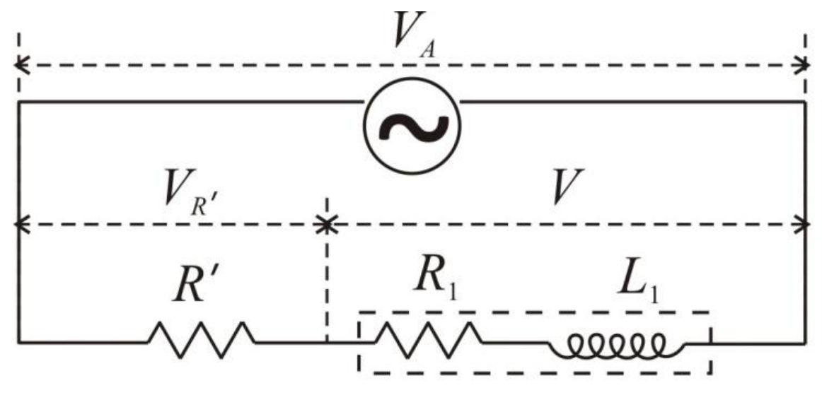
If the applied voltage across the series combination consisting of a known resistor with the coil is , then an expression relating applied voltage to the voltage drops across , across the coil and the angle is
All quantities except in Equation (6) are measurable.
Hence measuring the three voltages , and , and using Equations (4), (5) and (6), , and can be determined. Knowing the frequency of the alternating current the value of can be calculated.
Alternatively, from Equations (4) and (6) we can express the value of in terms of the three measured voltages as
The impedance of the coil can be calculated using the formula and the value of could be obtained from
Coupled Circuits
The energy supplied by the power source to the primary can be dissipated partially in the primary and the remainder in other mutually coupled secondaries. When no mechanical work is done, the energy dissipation is only in resistances. The inductances store energy in the magnetic field associated with them. With current (rms value) the average stored energy in inductance is equal to .
When a current flows in the secondary the emf induced due to it in the primary brings about change in the primary current. Seen from the primary side the effect is a consequence of change in the effective resistance and reactance of the primary coil and there is no need to know the parameters in the secondary circuit. The total energy dissipated in primary as well as secondary circuits appears as if it is dissipated in the effective primary resistance when seen from the primary side.
The effective values of resistance and inductance of primary can be related to a ‘reflected’ resistance and a ‘reflected’ inductance from the secondary side. The (average) power dissipated in the reflected resistance in the primary has to be equal to that in resistance in the secondary circuit. This gives
Similarly, we can relate the reflected inductance to the secondary inductance from
Considering the fact that the induced emf in the secondary due to an alternating primary current has magnitude equal to we can write the equation corresponding to Kirchhoff’s loop rule for the secondary in terms of rms values of primary and secondary currents as
where is the impedance of the secondary circuit. When the secondary impedance is infinite the mutually induced emf appears as the voltage across the open ends of the secondary.
APPARATUS:
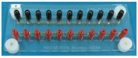
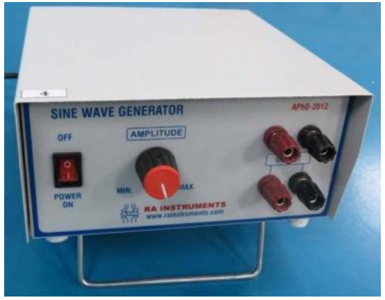
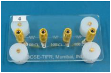
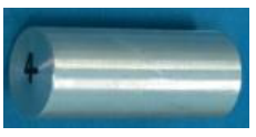
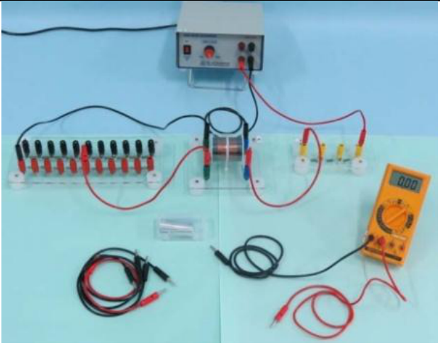
The apparatus provided for the experiment consists of the following.
- A sine wave generator with output of about 10 V (rms) at 1000 Hz frequency
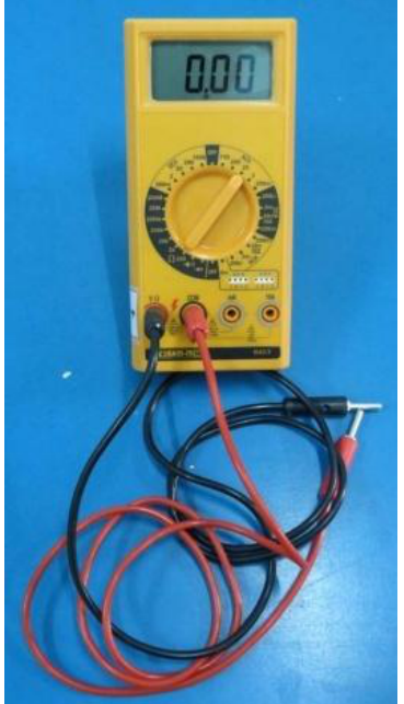
- A digital multimeter (DMM) to be used as a voltmeter
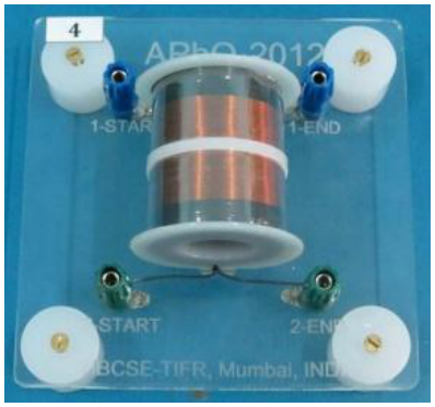
- A pair of coaxial coils wound one around the other on a cylindrical hollow piece of non magnetic non conducting bobbin
- A piece of aluminum rod capable of fitting inside the bobbin
- Two series of ten resistors mounted on an acrylic board: one consisting of 100 ohms resistors and the other of 10 ohm resistors with banana pin sockets
- The required resistance for load or sampling resistance can be selected using this resistance board and connecting wire pieces. A separate acrylic board with resistance of 300 ohms is provided which can be used for sampling resistor when the other board is used for load resistance.
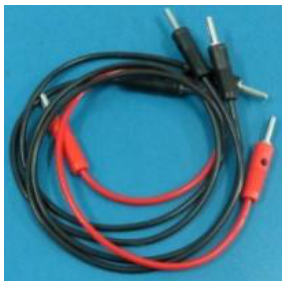
- A set of five red and five black wires with banana pins at their ends (the pair of longer red and black wires is meant for use as DMM probes).
The output of the sine wave generator of frequency 1000 Hz is to be used as the alternating source voltage. Use the 20 V range of the DMM to measure rms ac voltages.
The magnitudes of currents and when needed are to be calculated from the measured voltages across known values of in primary and in secondary respectively.
EXPERIMENT
PART 1: Determining Resistance and Inductance of a Coil with Air-core and Aluminium Core (3,4 т.)
Connect coil 1 (with blue terminals) in series with a resistor (to be selected from the resistance board) across the output terminals of the sine wave generator. The sine wave generator will be on before you start your experiment for stabilization of its output. Do not turn it off. Keep the output voltage amplitude maximum. (The DMM should show the output about 10 V).
The ac output of the generator may have some asymmetry. In that case, the readings of the DMM will show slightly different readings, when the input polarities of the DMM are interchanged between ‘V/Ω’ to ‘com’. To correct for the error due to asymmetry repeat each reading by interchanging the polarity of the probes of the DMM and take the mean of the two readings.
Choose the value of R´ to obtain and V approximately equal so that the systematic error in Z becomes negligible.
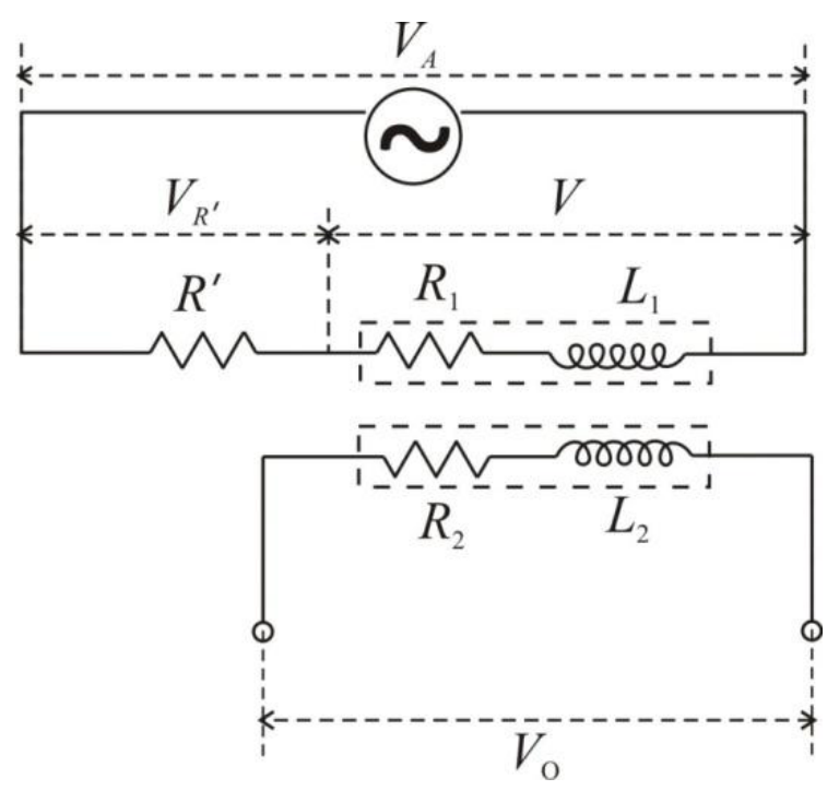
a) Measure the voltages , and as well as across the terminals of the other coil. Determine the resistance and inductance of coil 1 (with blue terminals) and estimate the uncertainties in the values determined. [0,9 т.]
b) Connect the other coil (coil 2 with green terminals), make the necessary measurements and determine and . Evaluate the uncertainties in the values obtained. [0,9 т.]
c) Now insert the piece of aluminium rod at the core of the coils and repeat the procedure to obtain the values of inductances * and resistance * and the uncertainties in them for coil1. [0,8 т.]
d) Make necessary measurements and determine inductance * and resistances, * of coil 2 when it has an aluminium core. Estimate the uncertainties in the values. [0,8 т.]
Note: Uncertainty calculations need not be done for parts 2, 3 and 4.
PART 2: Mutual Inductance and Coupling Constant (3 т.)
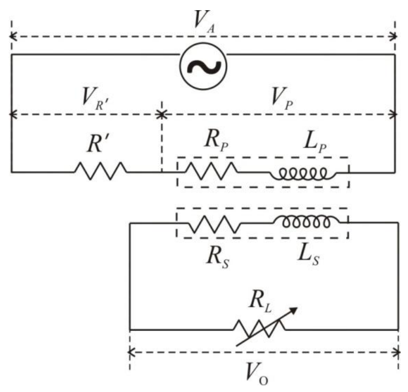
f) Mutual inductance can be obtained from the readings of and (recorded in Part 1). Find the average values for air core as well as aluminium core coils. The relation between the mutual inductance and the self inductances of the coupled coils is given by . Determine the value of , the coupling coefficient in the two cases. [0,4 т.]
g) Select coil 1 (with blue terminals) as primary and coil 2 (with green terminals) as secondary. Connect the primary in series with the sampling resistor ohm across the output terminals of the generator. Connect across the secondary the variable load . The output voltage is to be measured across . Change and measure the voltages , , and corresponding to each value of . [0,8 т.]
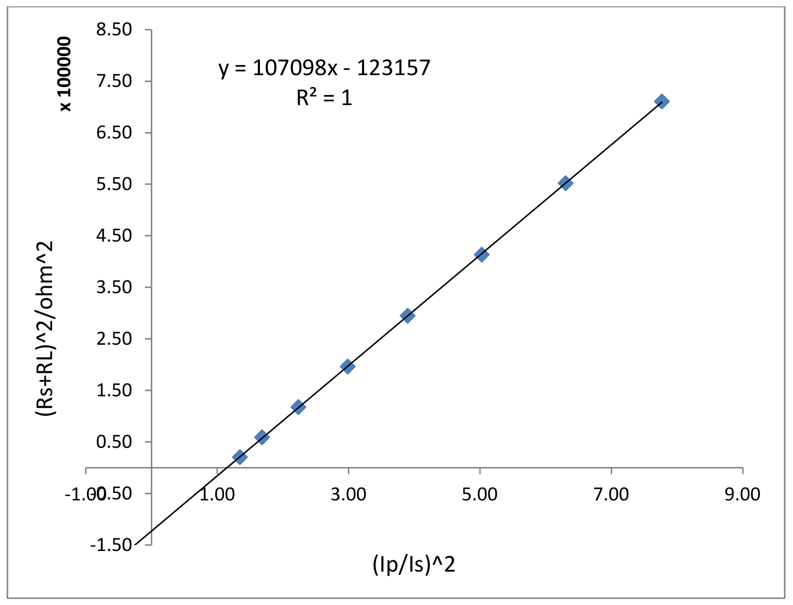
h) A linear graph can be plotted combining various terms appearing in Equation (10) written in expanded form. Write the linear expression for plotting a graph whose slope can be used to obtain the value of and intercept to obtain the value of secondary reactance . [0,2 т.]
i) Calculate the necessary quantities using data from (g) to plot the graph corresponding to the expression obtained in the step (h) above. [0,9 т.]
j) Plot the graph and obtain the values of and . [0,7 т.]
PART 3: Relations between Effective Primary Impedance and the Reflected Quantities from Secondary (2,4 т.)
k) Use the data collected in Part 2 to determine the effective resistance and the effective reactance of the primary corresponding to each value of in secondary. [0,6 т.]
l) Use the data of Part 2 to calculate the values of reflected resistance as defined in Equation (8) and of reflected reactance referring Equation (9) corresponding to the values of . [0,6 т.]
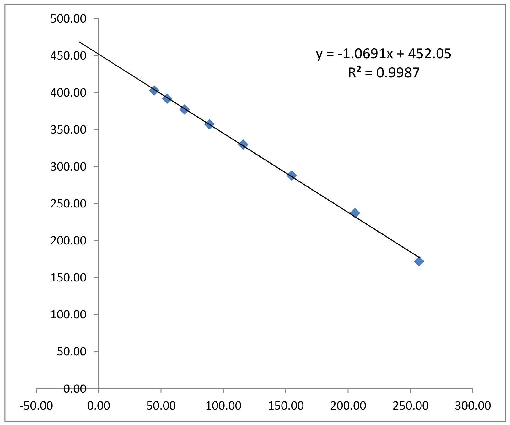
m) Plot graph of against . Taking into consideration the likely uncertainties of the quantities plotted write down the equation giving the relationship between the effective primary reactance and the reflected reactance. [0,6 т.]
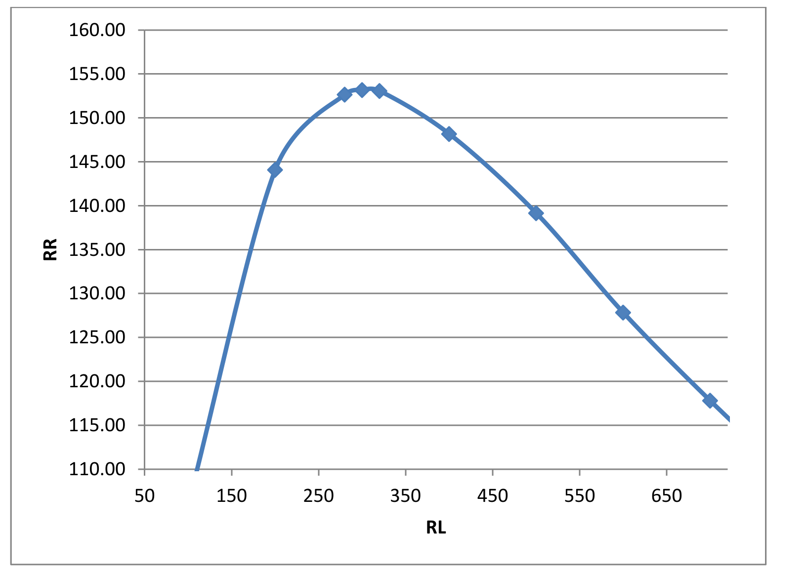
n) Represent graphically the relation between and over the range of study and find the value of for which the reflected resistance attains a maximum. If needed, take some more observations to supplement the observations in Part 2 for locating the point with greater precision. [0,6 т.]
PART 4: Eddy Current Effects (1,2 т.)
o) A model based on the analysis of the data in Part 3 suggests how to estimate the ratio of inductance and resistance seen by the eddy currents set up in the core of a coil connected to a power source.
The analysis of the data of Part 2(i) and (j) should show that . The relation between and is obtained from Part 3(m).
Refer to the data collected in Part 1(c) and estimate the ratio of inductance and resistance as seen by eddy currents in the aluminium core when the power supply is connected to coil 1 and coil 2 respectively. [0,8 т.]
p) Connect the coils as in Part 2 Fig.3 and insert the piece of aluminium rod at the core of the coils. Write down the expression giving the power loss in the aluminium core.
Set ohms and ohms. Adjust the magnitude of equal to 9.0 V. Make the necessary measurements and calculate the power dissipation due to the eddy currents in the aluminium core. [0,4 т.]
Отговори
PART 1: Determining Resistance and Inductance of a Coil with Air-core and Aluminium Core, a) R1 = 52.57, L1 = 71.43 mH; U(R) = 3.00, U(L) = 0.0002
Model-solution values (Part 1(a) table); a measured result depends on the set-up.
PART 1: Determining Resistance and Inductance of a Coil with Air-core and Aluminium Core, b) R2 = 42.96, L2 = 55.18 mH; U(R) = 2.00, U(L) = 0.0001
Model-solution values (Part 1b table); a measured result depends on the set-up.
PART 1: Determining Resistance and Inductance of a Coil with Air-core and Aluminium Core, c) R1 = 109.68, L1 = 43.72 mH; U(R) = 3.00, U(L) = 0.0002
Model-solution values (Part 1(c) table); a measured result depends on the set-up.
PART 1: Determining Resistance and Inductance of a Coil with Air-core and Aluminium Core, d) R2 = 71.48, L2 = 42.33 mH; U(R) = 3.00, U(L) = 0.0002
Model-solution values (Part 1(d) table); a measured result depends on the set-up.
PART 2: Mutual Inductance and Coupling Constant, f) Mavg (Air) = 53.00 mH, k = 0.844; M _avg (Al core) = 34.58 mH, k = 0.804
Model-solution values.
PART 2: Mutual Inductance and Coupling Constant, h)
PART 2: Mutual Inductance and Coupling Constant, j) Slope 1.07E+05, M = 52.08 mH; intercept 1.23E+05, X2 = 350.94 Ω
Model-solution values.
PART 3: Relations between Effective Primary Impedance and the Reflected Quantities from Secondary, m)
Model-solution fit: y = -1.0691x + 452.05, R² = 0.9987.
PART 4: Eddy Current Effects, o) Lc/Rc: Blue Coil 4.85E-04, Green Coil 4.50E-04
Model-solution values.
PART 4: Eddy Current Effects, p) 0.0165 W
Model solution: ΔP = 1.65E-02 W, with .
Решение
Model Solution
Part 1
Part 1(a):
| Coil Blue (1-1) | AIR CORE | f = 1.000 KHz | ||||||||||
|---|---|---|---|---|---|---|---|---|---|---|---|---|
| R' | V | Vo | ωM | M (mH) | (mH) | |||||||
| 450 | 10.090 | 6.760 | 6.770 | 4.940 | ||||||||
| 10.060 | 6.700 | 6.740 | 4.910 | |||||||||
| Avg | 450 | 10.075 | 6.730 | 6.755 | 4.925 | 0.015 | 451.67 | 52.57 | 448.60 | 329.31 | 52.44 | 71.43 |
| ΔVR' | ΔV | |
|---|---|---|
| 0.14 | 0.11 | 0.11 |
| us(z) | us( R) | ur(Z) | ur( R) | uc( R) | uc(Z) | uc(X) | uc(L) | U( R) | U(X) | U(L) |
|---|---|---|---|---|---|---|---|---|---|---|
| 0.0057 | 1.1432 | 0.2747 | 0.4235 | 1.2191 | 0.2748 | 0.3114 | 0.000050 | 3.00 | 0.7 | 0.0002 |
Part 1b:
| Coil Green (2-2) AIR CORE f = 1.000 KHz | ||||||||||||
|---|---|---|---|---|---|---|---|---|---|---|---|---|
| R' | V | Vo | ωM | M (mH) | (mH) | |||||||
| 350 | 9.960 | 6.690 | 6.610 | 6.390 | ||||||||
| 9.980 | 6.630 | 6.680 | 6.410 | |||||||||
| Avg | 350 | 9.970 | 6.660 | 6.645 | 6.400 | 0.019 | 349.21 | 42.96 | 346.56 | 336.34 | 53.56 | 55.18 |
| ΔVR' | ΔV | |
|---|---|---|
| 0.14 | 0.11 | 0.11 |
| us(z) | us( R) | ur(Z) | ur( R) | uc( R) | uc(Z) | uc(X) | uc(L) | U( R) | U(X) | U(L) |
|---|---|---|---|---|---|---|---|---|---|---|
| 0.0027 | 0.9057 | 0.2153 | 0.3335 | 0.9651 | 0.2153 | 0.2478 | 0.000039 | 2.00 | 0.5 | 0.0001 |
Part 1(c)
| Coil Blue (1-1) | Al CORE | f = 1.000 KHz | ||||||||||
|---|---|---|---|---|---|---|---|---|---|---|---|---|
| R' | V | Vo | ωM | M* (mH) | (mH) | |||||||
| 290 | 9.900 | 5.940 | 6.010 | 4.450 | ||||||||
| 9.880 | 5.890 | 6.050 | 4.410 | |||||||||
| Avg | 290 | 9.890 | 5.915 | 6.030 | 4.430 | 0.020 | 295.64 | 109.68 | 274.54 | 217.19 | 34.58 | 43.72 |
| ΔVR' | ΔV | |
|---|---|---|
| 0.14 | 0.10 | 0.10 |
| us(z) | us( R) | ur(Z) | ur( R) | uc( R) | uc(Z) | uc(X) | uc(L) | U( R) | U(X) | U(L) |
|---|---|---|---|---|---|---|---|---|---|---|
| 0.0220 | 1.2498 | 0.2030 | 0.3740 | 1.3046 | 0.2042 | 0.5657 | 0.000090 | 3.00 | 1.2 | 0.0002 |
Part 1(d):
| Coil Green (2-2) Al CORE f = 1.000 KHz | ||||||||||||
|---|---|---|---|---|---|---|---|---|---|---|---|---|
| R' | V | Vo | ωM | M*(mH) | (mH) | |||||||
| 280 | 9.860 | 6.280 | 6.170 | 4.840 | ||||||||
| 9.830 | 6.230 | 6.130 | 4.860 | |||||||||
| Avg | 280 | 9.845 | 6.255 | 6.150 | 4.850 | 0.022 | 275.30 | 71.48 | 265.86 | 217.11 | 34.57 | 42.33 |
| ΔVR' | ΔV | |
|---|---|---|
| 0.14 | 0.10 | 0.10 |
| us(z) | us( R) | ur(Z) | ur( R) | uc( R) | uc(Z) | uc(X) | uc(L) | U( R) | U(X) | U(L) |
|---|---|---|---|---|---|---|---|---|---|---|
| 0.0173537 | 0.9509 | 0.1821 | 0.3106 | 1.000 | 0.1829 | 0.329 | 0.000052 | 3.00 | 0.7 | 0.0002 |
Part 2
Part 2(f):
| (Air) = | 53.00 mH | k = | 0.844 | |
|---|---|---|---|---|
| (Al core) = | 34.58 mH | = | 0.804 |
Part 2(g):
| AIR Core | f = 1.000 KHz R'=300Ω | ||||||||||
|---|---|---|---|---|---|---|---|---|---|---|---|
| Sr. | V | Ip | Zp | Is | |||||||
| 1 | 100 | 10.19 | 5.99 | 4.97 | 1.73 | ||||||
| 10.15 | 6.03 | 4.94 | 1.72 | ||||||||
| Avg | 100 | 10.17 | 6.01 | 4.96 | 1.73 | 0.0200 | 247.34 | 177.56 | 172.19 | 0.017 | |
| 2 | 200 | 10.12 | 5.39 | 5.67 | 2.77 | ||||||
| 10.09 | 5.44 | 5.70 | 2.79 | ||||||||
| Avg | 200 | 10.11 | 5.42 | 5.69 | 2.78 | 0.0181 | 314.96 | 207.03 | 237.36 | 0.014 | |
| 3 | 300 | 10.13 | 5.17 | 6.17 | 3.44 | ||||||
| 10.15 | 5.11 | 6.19 | 3.43 | ||||||||
| Avg | 300 | 10.14 | 5.14 | 6.18 | 3.44 | 0.0171 | 360.70 | 216.93 | 288.18 | 0.011 | |
| 4 | 400 | 10.11 | 5.00 | 6.51 | 3.88 | ||||||
| 10.14 | 5.05 | 6.53 | 3.87 | ||||||||
| Avg | 400 | 10.13 | 5.03 | 6.52 | 3.88 | 0.0168 | 389.25 | 206.46 | 329.99 | 0.010 | |
| 5 | 500 | 10.15 | 4.93 | 6.74 | 4.20 | ||||||
| 10.12 | 4.99 | 6.77 | 4.17 | ||||||||
| Avg | 500 | 10.14 | 4.96 | 6.76 | 4.19 | 0.0165 | 408.57 | 198.08 | 357.34 | 0.008 | |
| 6 | 600 | 10.10 | 4.98 | 6.91 | 4.42 | ||||||
| 10.13 | 4.91 | 6.93 | 4.40 | ||||||||
| Avg | 600 | 10.12 | 4.95 | 6.92 | 4.41 | 0.0165 | 419.82 | 183.87 | 377.41 | 0.007 | |
| 7 | 700 | 10.14 | 4.97 | 7.05 | 4.58 | ||||||
| 10.11 | 4.91 | 7.07 | 4.60 | ||||||||
| Avg | 700 | 10.13 | 4.94 | 7.06 | 4.59 | 0.0165 | 428.74 | 173.76 | 391.96 | 0.007 | |
| 8 | 800 | 10.09 | 4.91 | 7.17 | 4.74 | ||||||
| 10.12 | 4.98 | 7.15 | 4.72 | ||||||||
| Avg | 800 | 10.11 | 4.95 | 7.16 | 4.73 | 0.0165 | 434.38 | 161.90 | 403.08 | 0.006 |
Part 2(h)
| Slope | M | |
|---|---|---|
| 1.07E+05 | 52.08 mH | |
| Intercept | ||
| 1.23E+05 | 350.94 Ω |
Part 2(i)
| 1.35 | 20438.25 |
| 1.69 | 59030.73 |
| 2.24 | 117623.21 |
| 2.99 | 196215.69 |
| 3.90 | 294808.17 |
| 5.03 | 413400.65 |
| 6.31 | 551993.13 |
| 7.77 | 710585.61 |
Part 2(j):
Part 3
Part 3(k) and 3(l):
| Sr. | ||
|---|---|---|
| 1 | 106.00 | 256.95 |
| 2 | 144.08 | 205.52 |
| 3 | 153.17 | 154.78 |
| 4 | 148.17 | 115.92 |
| 5 | 139.16 | 88.82 |
| 6 | 127.84 | 68.91 |
| 7 | 117.81 | 54.95 |
| 8 | 108.46 | 44.59 |
Part 3(m)
Inference:
Part 3(n):
| Sr. | V | Vo | Ip | Is | |||||
|---|---|---|---|---|---|---|---|---|---|
| 1 | 280 | 10.06 | 5.11 | 6.05 | 3.29 | ||||
| 10.03 | 5.16 | 6.03 | 3.30 | ||||||
| 280 | 10.05 | 5.14 | 6.04 | 3.30 | 0.0171 | 0.01 | 2.12 | 152.65 | |
| 2 | 320 | 10.02 | 5.09 | 6.19 | 3.51 | ||||
| 10.05 | 5.03 | 6.21 | 3.50 | ||||||
| 320 | 10.04 | 5.06 | 6.20 | 3.51 | 0.0169 | 0.01 | 2.37 | 153.07 |
| RR | |
|---|---|
| 100 | 106.00 |
| 200 | 144.08 |
| 280 | 152.65 |
| 300 | 153.17 |
| 320 | 153.07 |
| 400 | 148.17 |
| 500 | 139.16 |
| 600 | 127.84 |
| 700 | 117.81 |
| 800 | 108.45771 |
Part 4
Part 4(o):
| Blue Coil | Green Coil |
|---|---|
| Lc/Rc | Lc/Rc |
| 4.85E-04 | 4.50E-04 |
Part 4(p)
| V | Vo | ||||||||
|---|---|---|---|---|---|---|---|---|---|
| 1000 | 9.00 | 5.32 | 5.08 | 3.45 | |||||
| 9.01 | 5.27 | 5.10 | 3.43 | ||||||
| Avg | 1000 | 9.01 | 5.30 | 5.09 | 3.44 | 0.0177 | 0.003 | 145.23 | |
| Δ P = | 1.65E-02 W |
Оригинал в Архива: exp2.pdf · официални решения: exp2_sol.pdf