Съдържание
УсловиеExperiment A — Basic measurement (3 т.)Experiment B — The resonant method to measure the piezoelectric coefficient (4,5 т.)Experiment C — The Curie temperature of the PZT plate (4 т.)Experiment D — Application: measuring the speed of sound in aluminum (6,5 т.)Experiment E — Application: locating a defect in an aluminum rod (2 т.)Answer SheetsРешениеAPhO 2015, Експеримент — Experiment Problem. The Piezoelectric Effect And Its Applications
Experimental Competition — The Piezoelectric Effect And Its Applications · 7 май 2015 г. · 20 т.
Внимание: Бележка към темата
The archive catalogue lists five headings; they are connected sections A–E of one 20-point experiment. All 17 original blank answer sheets are retained. In the B answer sheets, numbering and marks differ from the question booklet and marking scheme; the additional coefficient-derivation request has no obtained derivation key. Separate Additional Writing Sheets mentioned in the instructions were not obtained.
Native answer-sheet companion — Experimental Competition, May 7, 2015, 08:30–13:30 hours. These are the complete unfilled original forms, including blank working areas and all five original plotting grids. The cover contains STUDENT CODE boxes, “Additional number of writing sheets=”, “Do not write below this line”, and the maximum marks Part A 3.0 / Part B 4.5 / Part C 4.0 / Part D 6.5 / Part E 2.0 / Total 20.0; Marks scored is blank. Every following page has Country/Student Code fields.
Source-edition difference in B: form page 4 prints B.1 “Prove that the equivalent circuit has a resonant frequency and an antiresonant frequency .” (0.9 pts). Page 5 prints B.2 “Derive from and other known parameters of the PZT plate.” (0.5 pts). Page 6 prints B.3 the current/frequency measurement request (3.1 pts), with its blank plotting grid on page 7. These differ from question/marking-scheme B.1 (1.0 pts) and B.2 (3.5 pts). The extra form-only coefficient-derivation request has no obtained derivation key; question page 14 supplies the coefficient formula. It remains an attributed original variant, without an invented official answer.
The other forms repeat the corresponding native A.1/A.2,C.1/C.2,D.1–D.5,E.1/E.2 requests and points. Page 9 has the C.2 blank grid; page 10 is its blank continuation; page 12 has D.2 grid; page 14 has D.4 grid; page 16 has E.1 grid. No unfilled field is replaced by sample-key data.
Additional Writing Sheets mentioned by question page 2 are not a separate obtained companion in the complete three-file archive folder.
Source scoring discrepancy: The printed A.1 marking rubric on native solution page 2 states Total: 1.6, while its listed positive awards sum to 1.7 (0.2 + 0.2 + 0.3 + 0.3 + 0.3 + 0.2 + 0.2). The printed total, individual awards and penalties are retained without changing the official scoring.
Native cover and competition instructions
16th ASIAN PHYSICS OLYMPIAD 2015 — 3rd–11th MAY, HANGZHOU, CHINA. Experimental Competition, May 7, 2015, 08:30–13:30 hours. Experiment Problem. There are 22 pages including the cover page.
Please first read the following instructions carefully:
- The time available is 5 hours for the experimental problem.
- Use only the pen and equipment provided.
- There is a set of Answer Sheets in which you have to enter your data and results.
- Write down your Student Code in the boxes at the top of each Answer Sheets and additional sheets which you submit.
- Additional Writing Sheets are provided.
- If you use any additional Writing Sheets, please write down your Student Code, the Question Number and the Page Number on these additional Writing Sheets.
- If you use additional Writing Sheets that you do not wish to be marked, put a large ‘X’ across the entire sheet.
- You should use mainly equations, numbers, symbols, graphs, figures and as little text as possible in your answers. Use the symbols defined in the question.
- At the end of the experiment arrange all sheets in the following order: a. Main Answer Sheets; b. Used Writing Sheets; c. Writing sheets which are marked with ‘X’; d. Unused Writing Sheets; e. The question paper.
- Put all the papers inside the envelope and leave the envelope on your desk.
- You are not allowed to take any sheet of paper or any material used in the experiment out of the room.
Условие
1. Introduction
The piezoelectric effect refers to the process that the electric charge accumulates in solid materials in response to applied mechanical stress (see Figure 1(a)). It is reversible, which means that materials exhibiting the piezoelectric effect also exhibit the converse piezoelectric effect, i.e., the internal generation of a mechanical strain resulting from an applied electrical field (see Figure 1(b)).
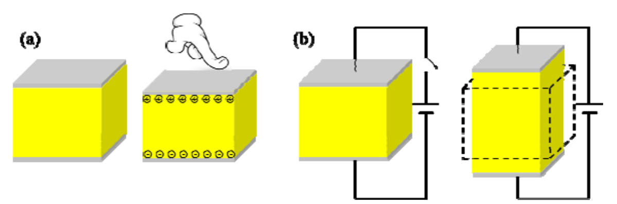
The piezoelectric materials are used in various applications covering a wide range from industrial and manufacturing to daily life, such as the production and detection of sound, generation of high voltages, microbalances, ultra-fine focusing of optical assemblies, ignition source for cigarette lighters, push-start propane barbecues, and quartz watches.
In addition to applications mentioned above, the piezoelectric materials are also actively used in scientific research. As very high electric fields correspond to only tiny changes in the dimensions of the piezoelectric materials, the piezoelectric materials become the most important tool for positioning objects with extreme accuracy. They are the basis of some commonly used tools in surface science, the scanning tunneling microscope (STM) and its variants. The 1986 Nobel Prize in physics was awarded to Gerd Binnig and Heinrich Rohrer for their design of STM.
Another merit of the piezoelectric materials is that they could enable conversion of signals between different modes such as mechanical, electrical and optical. With the help of ultra-low temperatures and state-of-the-art electronics, researchers are able to cool down the mechanical mode to its ground state and observe the quantization of motion. The experiment of creating such a quantum machine, a mechanical resonator made by piezoelectric aluminum nitride, was titled “Breakthrough of the Year 2010” by Science magazine.
There are many piezoelectric materials, both natural and synthetic. Some naturally occurring materials include quartz, bone and silk. Synthetic materials include ceramics, semiconductors and polymers. Lead zirconate titanate (), known as PZT, is the most common piezoelectric ceramic in use today, which exhibits strong piezoelectricity.
In this APhO2015 experiment, we will explore properties of PZT and its applications. For a given PZT plate, we will measure its piezoelectric coefficient via the resonant method and will estimate its Curie temperature by linear extrapolation. We will make a transducer out of a PZT plate to produce mechanical motions and sound waves in the medium; we will make a sensor out of a PZT plate for sensing the strength of sound waves. With the hand-made transducer and senor, we will measure the longitudinal and transverse wave velocities of sound in an aluminum rod. Finally, we will use sound waves to resonantly locate an artificially-designed defect in another aluminum rod.
2. General Safety Precautions:
- Be sure to switch off the equipment before plug in/out its power cord. Otherwise damage can occur.
- Do not turn on the thermostat water bath if the heating unit is not covered by water.
- Be careful not to spill the water onto nearby electronics and the electrical power socket.
- Be careful of the hot water.
- Be careful of electric shock.
- Do not drink/consume any of the materials provided for the experiment.
3. Apparatus
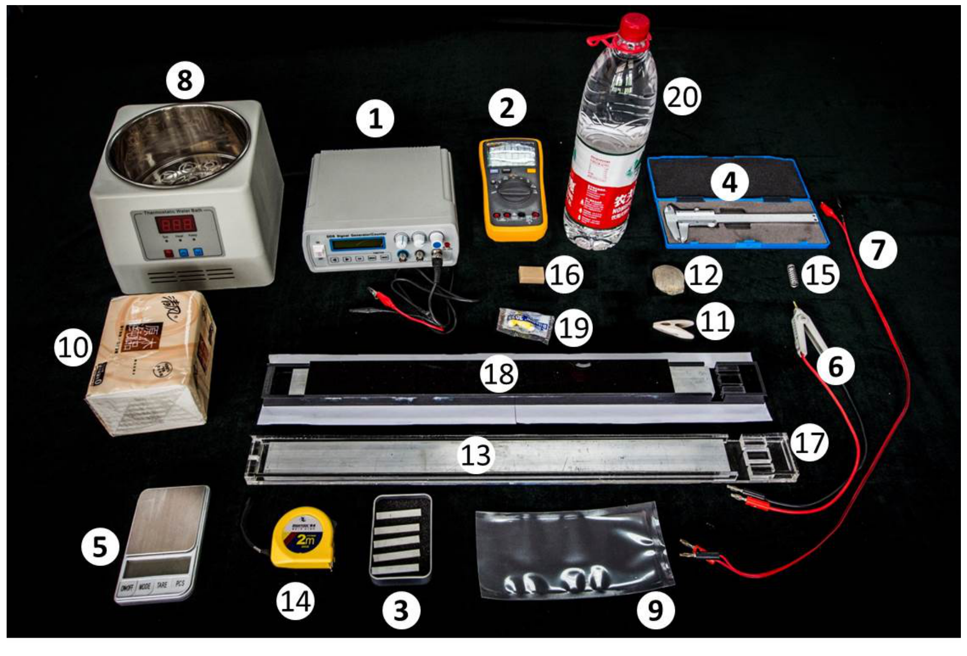
| Number | Apparatus |
|---|---|
| 1 | A signal generator which can output simple repetitive electrical waveforms over a wide range of frequencies. |
| 2 | A digital multimeter (DMM). |
| 3 | 5 PZT plates. Two flat surfaces of each plate are coated by thin films of silver. |
| 4 | A Vernier caliper. |
| 5 | An electronic weighing scale. |
| 6 | A Kelvin clip. The Kelvin clip features a crocodile clip with two isolated jaws, which are connected to two banana plugs respectively. It is used to clamp a PZT plate. |
| 7 | A cable with two banana plugs connecting to two crocodile clips, respectively. One jaw of each crocodile clip is wrapped by a black tube, and therefore it is important to have the correct polarity when clamping. |
| 8 | A thermostat water bath. |
| 9 | A plastic bag. |
| 10 | Paper towels. |
| 11 | A plastic clip. |
| 12 | A pebble. |
| 13 | An aluminum rod. |
| 14 | A steel tape measure. |
| 15 | A spring. |
| 16 | An eraser. |
| 17 | A transparent plastic box to accommodate the aluminum rod and the PZT plates together. |
| 18 | A black plastic box with an aluminum rod inside. A defect, invisible from outside the box, is artificially engineered at a spot along the rod. |
| 19 | A pair of earplugs. |
| 20 | 1.5 L bottled water. |
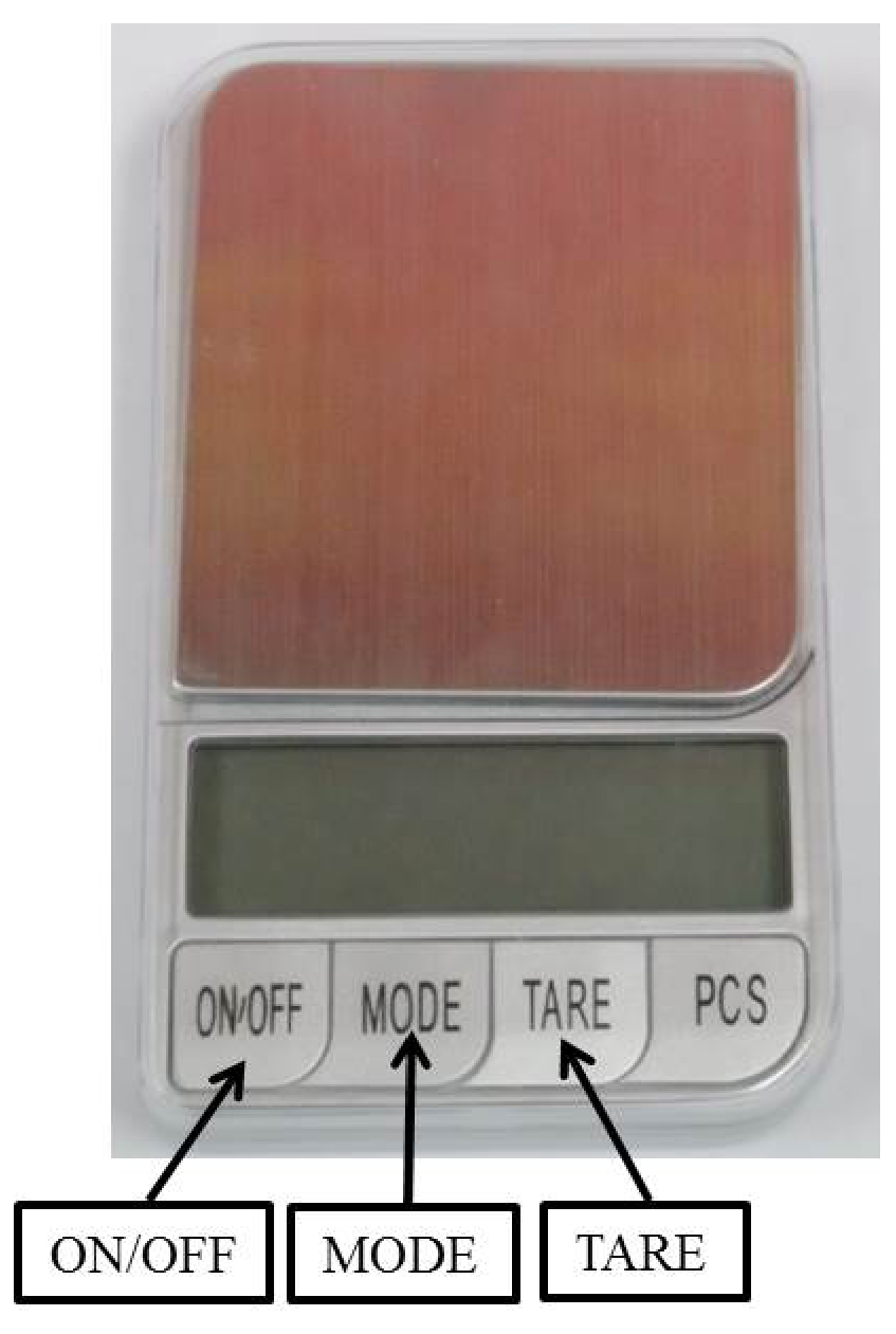
Instructions for the electronic weighing scale (see Figure 2)
- Place the scale on a flat, very stable surface.
- Press the “ON/OFF” button to turn on the scale.
- Wait until the reading is stable. If the reading is not zero, press the “TARE” button to re-Zero it.
- Press the “MODE” button to toggle units between “g”, “gn”, “oz”, “ozt”, “dwt”, “ct” and “tl”. It is recommended that you use the unit “g” (gram).
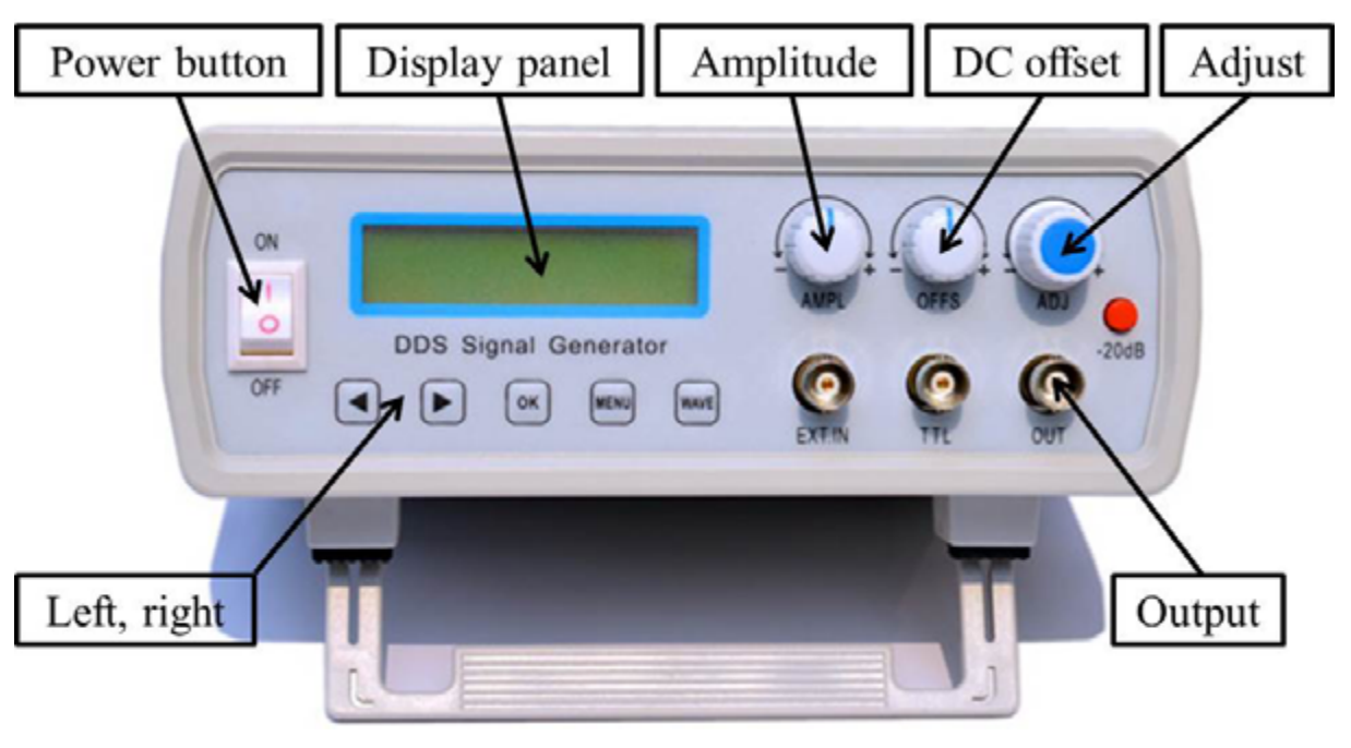
Instructions for the signal generator (see Figure 3)
- To turn on the machine, connect the detachable USB power cord (with the AC adapter) to the rear panel receptacle and turn on the front panel power button.
- The “Display Panel” shows the wave frequency and the wave type (sine, square, or triangle). We recommend sine for the experiment.
- Use the “Amplitude” knob to adjust the signal amplitude. Use the “Adjust” knob to change the signal frequency. Use the “◄” or “►” button to move the cursor.
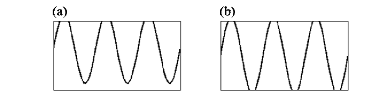
- Be careful when tuning the “DC offset” knob.his knob changes the DC offset of the signal. A big DC offset may cause signal clipping (see Figure 4 (a)). It is recommended that you calibrate the DC offset before using the signal generator: while using the DMM to monitor the DC voltage of the output, adjust the “DC Offset” knob until the DC voltage reaches zero.
- It is also recommended that you do not tune the “Amplitude” knob to maximum to avoid signal clipping (see Figure 4 (b)). You can tune the output amplitude to 3.0 V (rms) for the experiment: while using the DMM to monitor the AC voltage of the output at a frequency of, e.g., 1 kHz, adjust the “Amplitude” knob until the AC voltage reaches about 3.0 V (rms).
- If you press a button by mistake and do not know how to return to the original configuration, restart the machine to restore to default configuration.
Instructions for the digital multimeter (DMM. See Figure 5)
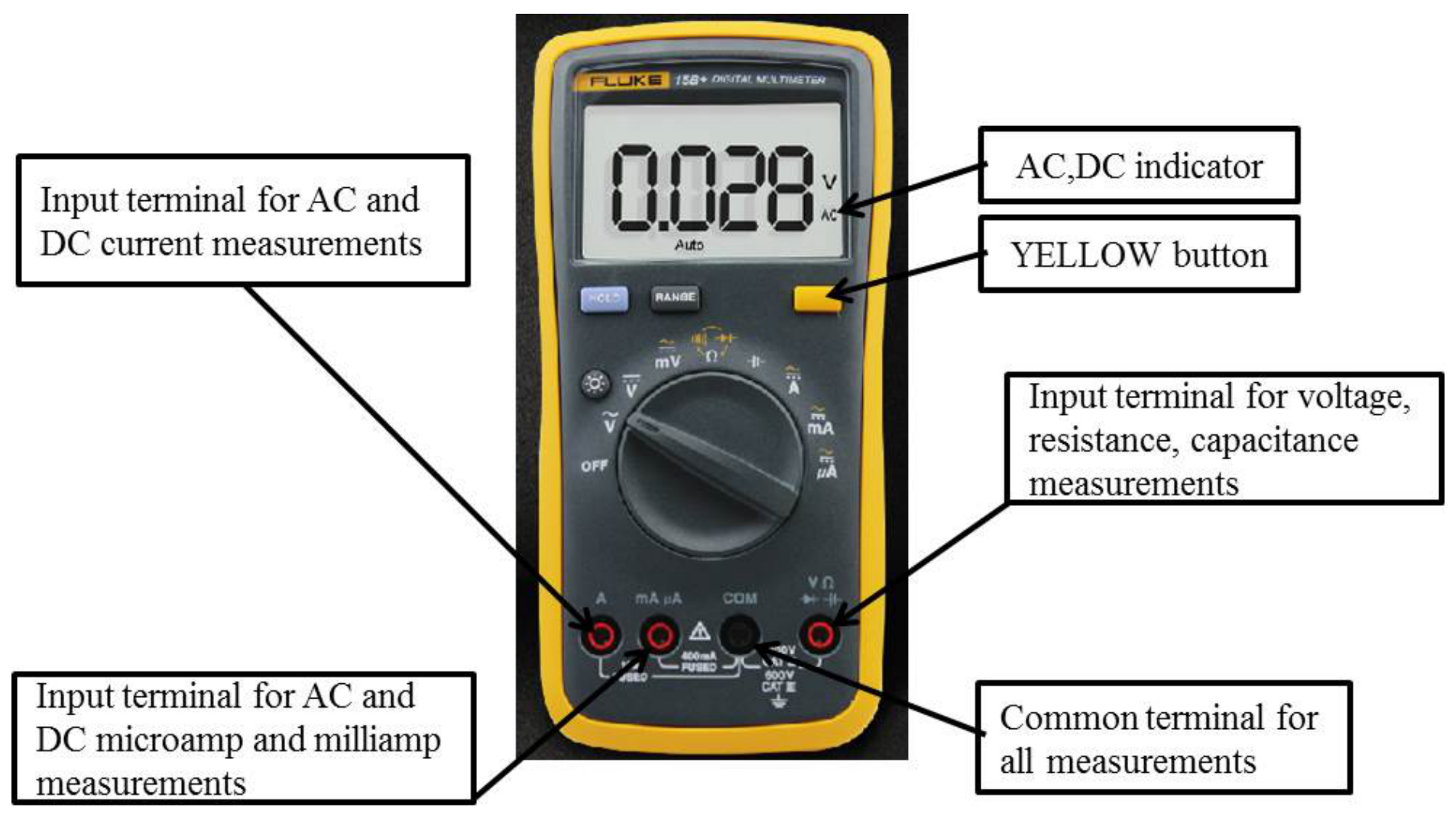
- Use the “VΩ” and “COM” inlets for measuring voltage, resistance and capacitance.
- Use the “mA” and “COM” inlets for measuring current.
- Use the rotary switch to select the proper function and measuring range.
- Toggle between the AC and DC modes by pressing the YELLOW button.
- The DMM enters the “Sleep mode” and blanks the display if the DMM remains inactive for more than 20 minutes. Turn the rotary switch to OFF and back to wake up the DMM. To disable the Sleep mode, hold down the YELLOW button while turning the DMM on.
- Attention: although it is usable for the experiment with frequencies up to 40 kHz, the DMM is not designed for accurately measuring the amplitude values of AC signals above 1 kHz. To calibrate the output voltage of the signal generator using the DMM, you should set the signal frequency to 1 kHz or below.
Instructions for the thermostat water bath (see Figure 6)
- Surfaces can become hot during use.
- It is strictly prohibited to turn on the machine if the heating unit is not covered by water.
- Be careful not to spill water onto the nearby electronics and the power socket.
- Fill in bottled water for the bath to be about half full. Properly connect the power cord and turn the bath on.
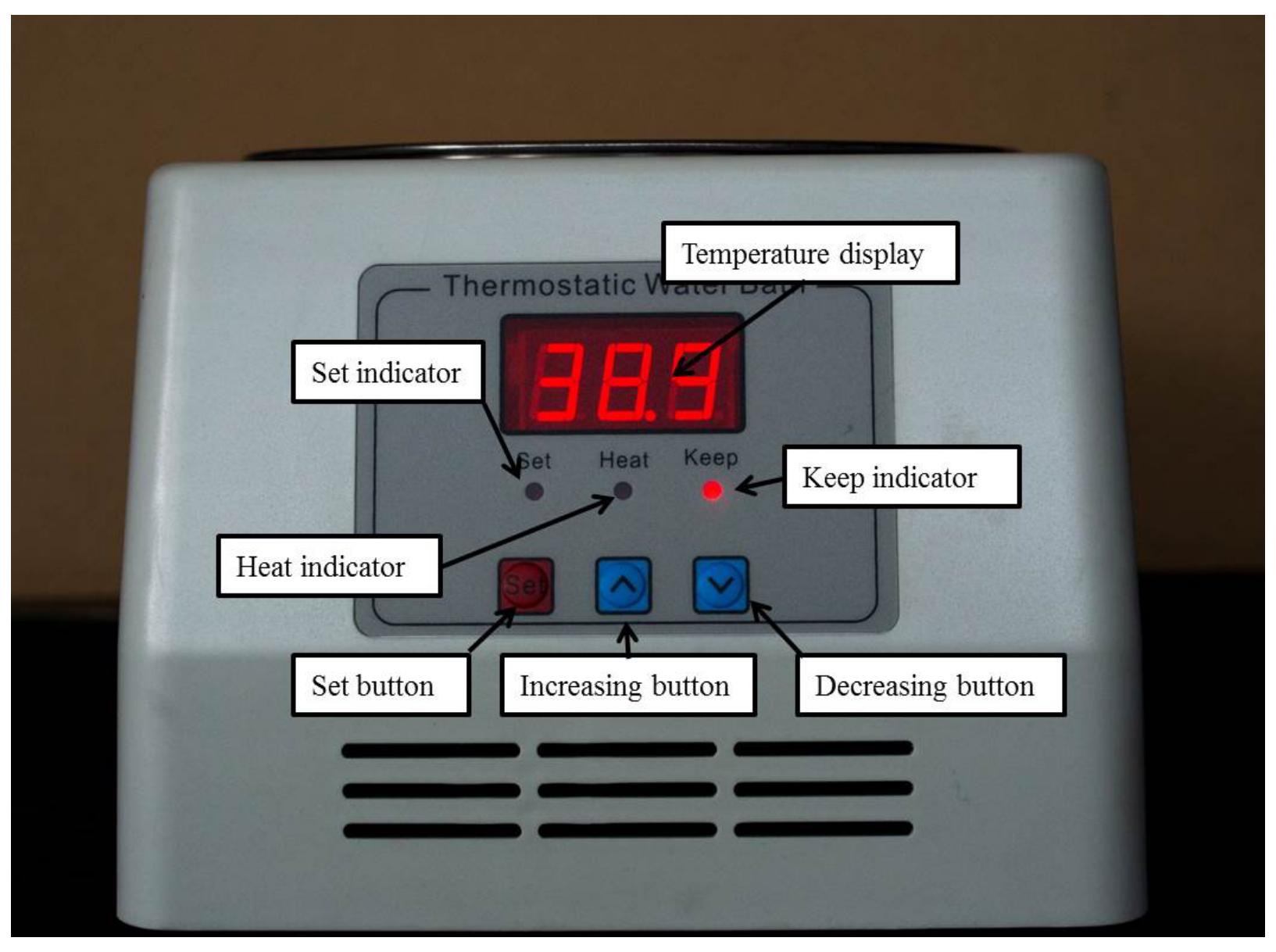
- To set the target temperature, press the “Set” button to enter the “Set” mode and the “Set” indicator will illuminate. Use the “Increasing” (“Decreasing”) button to increase (decrease) the displayed value to the target temperature. Press the “Set” button again to exit the “Set” mode and the water bath will start heating automatically. Check the “Temperature display” for actual temperature readings.
- During heating, the “Heat” indicator illuminates. After reaching the set temperature, the “Keep” indicator will illuminate and heating will stop.
- It is recommended that you ramp up the temperature gradually from low to high during the experiment.
Experiment A — Basic measurement (3 т.)
In this experiment, you are required to measure the dimensions, the mass and the capacitance of a PZT plate, and then calculate its density and relative permittivity .
Please choose a PZT plate. You are supposed to perform Experiments A, B and C using this same plate.
In Experiments A to E, error analysis is required if it is explicitly stated; it is not required if it is not stated.
A.1 Choose a PZT plate and use the Vernier caliper to measure its length , width and thickness . Use the electronic weighing scale to measure its mass . Use the DMM and the Kelvin clip to measure its capacitance (at ambient temperature).
Considering the slight non-uniformity in the dimensions of the PZT plate and the uncertainties of instrumental readings, repeat each measurement several times and then calculate the mean and the standard error. [1,6 т.]
Attention: The relative permittivity of the PZT plate is temperature dependent (see Experiment C). You are supposed to perform the capacitance measurement at ambient temperature. Avoid the direct warming up of the plate by your hand.
A.2 Now calculate the density and the relative permittivity of the PZT plate. Based on standard errors obtained from A.1, carry out the error analysis to estimate the uncertainties of and (vacuum permittivity ). [1,4 т.]
Experiment B — The resonant method to measure the piezoelectric coefficient (4,5 т.)
As described in the introduction section, the piezoelectric plate produces distortion (also called strain ) when subjected to an electric field. The proportional coefficient of the strain versus the electric field strength is defined as the piezoelectric coefficient
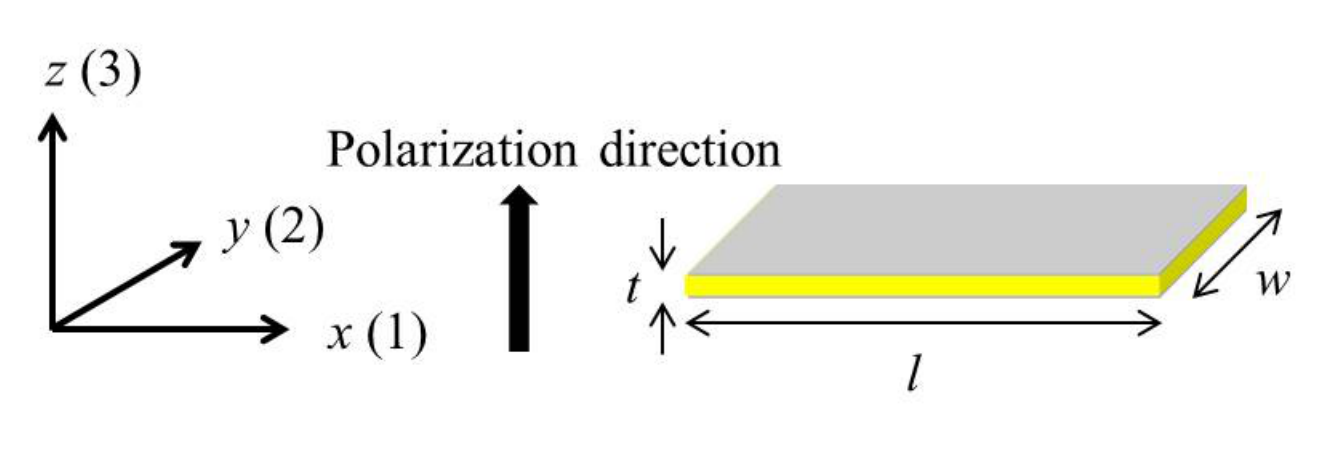
In reality, the PZT plate is anisotropic. There is a special direction called the polarization direction. During production of the PZT plate, a strong DC electric field is applied along its thickness direction (-axis in Figure 7) to align the molecular dipoles of the ceramic at a temperature higher than the Curie temperature (see Experiment C). This polarization remains after temperature is reduced below the Curie temperature and then the DC electric field is removed.
The top and bottom flat surfaces of the plate are coated with silver films as electrodes (see Figure 7). The electric field is along -axis (3) when the electrodes are connected to a voltage source, and we shall denote it as . Here we define
where and are strains along -axis (1) and -axis (3), respectively. Note that the strain is not necessarily parallel to the electric field . For PZT materials, is roughly half of . According to the parameters in Experiment A, it can be shown that length changes the most when a voltage is applied across the electrodes, i.e.,
where . To simplify the theoretical treatment, for such a long thin plate, vibrations along the width (-axis) and thickness (-axis) directions can be neglected and the problem reduces to a one-dimensional vibration problem. As such we remove the redundant subscript and simply denote as . In Experiments D and E the ignored vibration along the width (-axis) direction may cause slight imperfection to the measurement.
The PZT plate performs like a pure capacitor (with a capacitance from A.1) when driven by low-frequency signals. However, as frequency increases, the vibration of the PZT plate changes its circuitry behavior significantly. At certain frequencies, called resonant frequencies, the plate vibrates strongly and its impedance reaches a minimum. Along with the resonant frequencies, there are also frequencies where the impedance reaches a maximum, and we call them antiresonant frequencies.
The first resonant frequency of the plate is associated with its fundamental vibration mode along the length direction (-axis). Near , the PZT plate can be approximated by a simple circuit, with two capacitors ( and ) and an inductor () being arranged as shown in Figure 8.
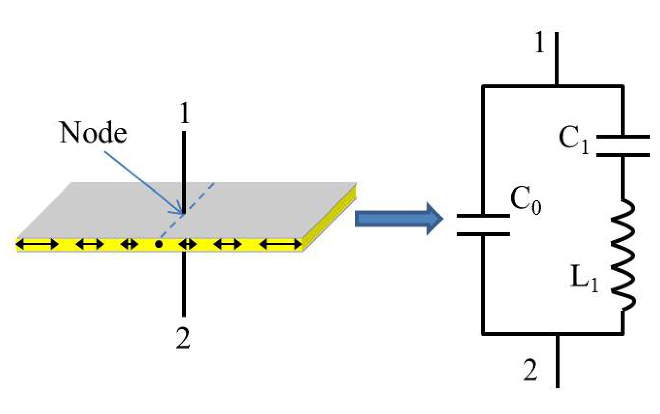
B.1 Derive the expressions for the resonant frequency and the antiresonant frequency of the equivalent circuit. [1 т.]
The piezoelectric coefficient can be calculated by the following formula
Now we perform the experiment to locate and . See the circuit schematics in Figure 9. We keep the output amplitude (the voltage ) of the signal generator constant, such that the impedance of the PZT plate correlates with the AC current in the circuit.
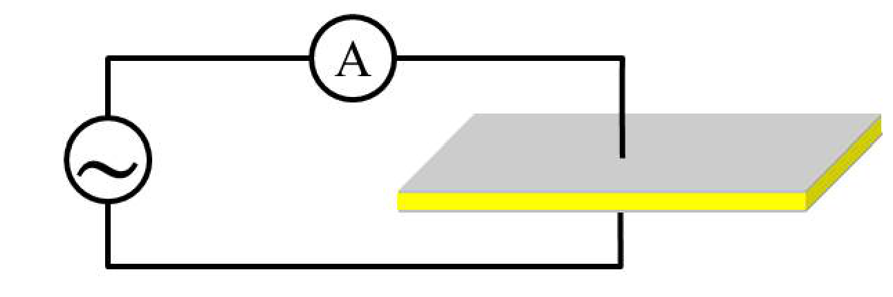
B.2 Measure the AC current through the PZT plate as a function of the signal frequency . Draw the - curve and find the resonant frequency and the antiresonant frequency . Calculate the piezoelectric coefficient accordingly. [3,5 т.]
Instructions:
(1) Connect the signal generator, the DMM and the PZT plate according to Figure 9. Note that the PZT plate should be clamped at the middle point along the length direction using the Kelvin clip, since the middle point is the node under the free boundary condition.
(2) The amplitude of the output signal changes little with frequency if the “Amplitude” knob of the signal generator remains untouched. However, the DMM may not respond to signals with a frequency above 40 kHz. Data above 40 kHz are not required.
(3) Attention: keep the clamped PZT plate intact during the experiment. Slight movement may cause drifting of the current reading.
(4) Attention: as mentioned in A.1, you are supposed to perform the measurement at ambient temperature. Avoid the direct warming up of the plate by your hand.
(5) Attention: if you do not hear any high pitch sound from your testing plate after sweeping frequency and you are confident with your measurement setup, you should contact the organizer as your instruments might be faulty.
Experiment C — The Curie temperature of the PZT plate (4 т.)
Most insulators have a dielectric susceptibility which is insensitive to the temperature variation. However, the static relative permittivity of the PZT ceramics changes with temperature according to the relation
Here and are constants independent of temperature. This relation is known as the Curie-Weiss law. Parameters and are called the Curie constant and the Curie temperature respectively, named after Pierre Curie.
A phase transition occurs at the transition temperature, . Above , the substance is in the paraelectric phase, in which the elementary dipoles of the various unit cells in the crystal are oriented randomly. Below , the elementary dipoles interact with each other, giving rise to an internal field, which lines up the dipoles. A spontaneous polarization appears in the absence of an applied electric field. The relative permittivity below is given as
From Experiment A we know that . We can ignore the constant term to obtain an approximation of the static relative permittivity as
Therefore capacitance of the PZT plate obtained from A.1 could vary with temperature as well. Since the Curie temperature of the PZT plate is much higher than the boiling temperature of water, we will estimate its Curie temperature by linear extrapolation.
C.1 Now measure the capacitance of the PZT plate at various temperatures and record the data. [1,5 т.]
Instructions:
(1) Use the cable with two banana plugs and two crocodile clips to connect the PZT plate to the DMM. Pay attention to the polarity of the two crocodile clips when clamping the PZT plate. Do not use the Kelvin clip because its ABS plastics will soften when heated.
(2) Put the PZT plate inside the plastic bag. Use the plastic clip to clamp the cable and the bag. Warning: one side of the bag is open. Do not tear the other side!
(3) Pour the 1.5 L bottled water into the water bath. Immerse the plastic bag in the water. Use the pebble to keep the plastic bag in the water.
(4) Turn on the water bath and set the target temperature. Warning: it is strictly prohibited to turn on the machine if the heating unit is not covered by water.
(5) Warning: be very careful with the hot water in the water bath. Remember that water at temperatures higher than can cause burns. For safety please do not set the temperature higher than .
(6) The temperature will rise slowly. Please record the capacitance of the PZT plate at different temperatures.
(7) Turn off the water bath and unplug the power cord from the power socket when the measurement is finished.
(8) Hint: to speed up the experiment, you can choose to set the target temperature to and record the capacitance as the temperature rises.
C.2 Analyze the data, draw a proper plot and calculate the Curie temperature accordingly. [2,5 т.]
Experiment D — Application: measuring the speed of sound in aluminum (6,5 т.)
In solids, sound can be transmitted as both longitudinal waves and transverse waves. The medium movements responsible for the two types of waves are illustrated below.
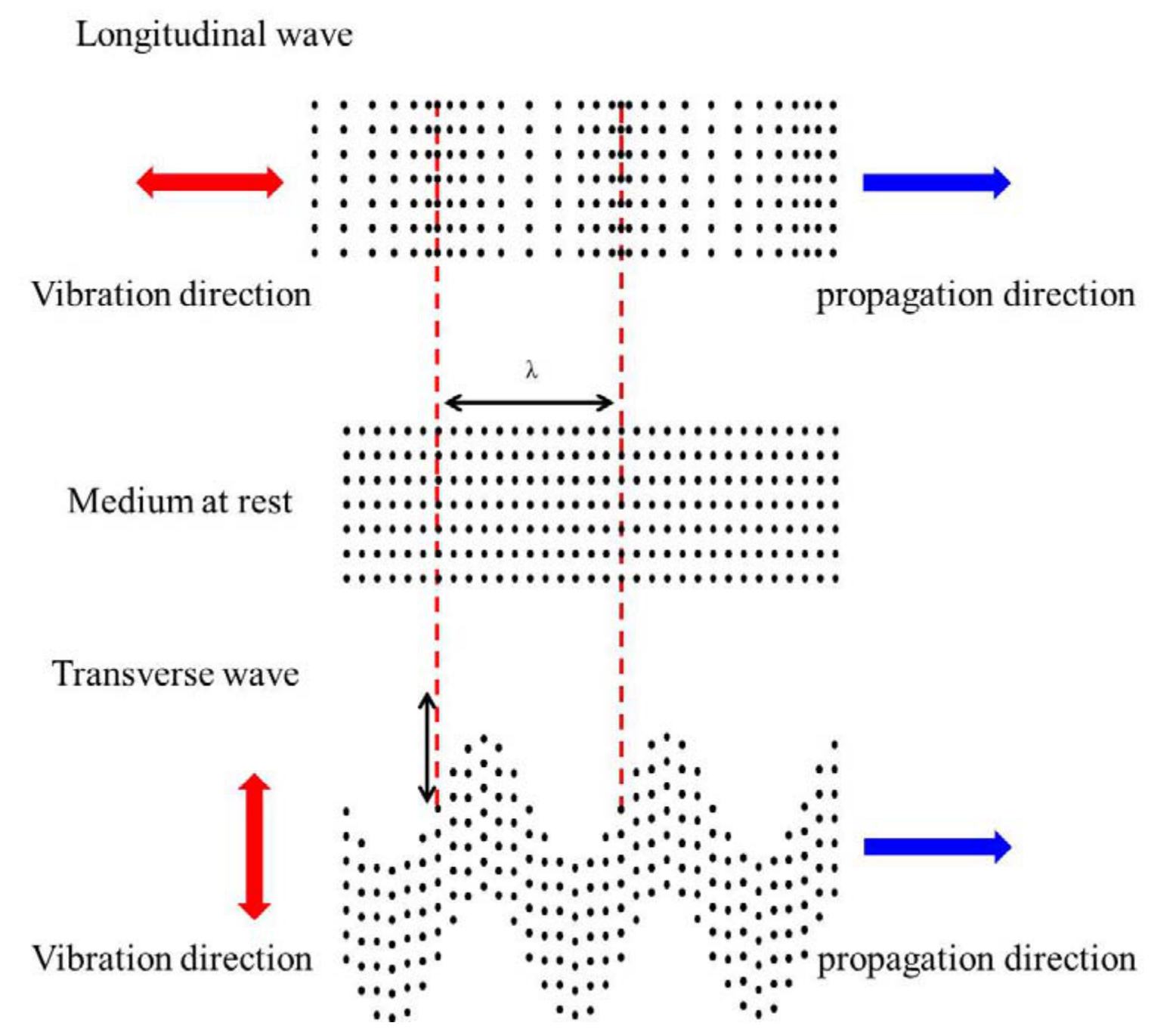
In longitudinal waves, oscillation occurs in the longitudinal direction or the direction of wave propagation. Longitudinal waves can be generated in liquids, as well as in solids because the energy travels through the atomic structure by a series of compression and expansion movements.
In transverse waves, displacement of the medium is perpendicular to the direction of wave propagation. Transverse waves require a solid medium for propagation, and cannot effectively propagate in liquids or gasses.
In this experiment, we will measure the longitudinal and transverse wave velocities of sound in an aluminum rod. We will first measure the transverse wave velocity, and then the longitudinal wave velocity.
D.1 Assume that the length of the aluminum rod is and the wave velocity is . Under the free boundary condition, derive the equation for the frequencies of the standing (resonant) waves along the long rod. Then derive the equation for the wave velocity from . [0,6 т.]
Now, we use a PZT plate as a transducer to produce sound waves in the aluminum rod, and use another PZT plate as a vibration sensor to detect the reflected sound waves.
First we measure the transverse wave velocity. As discussed in Experiment B, the vibration along the length direction is dominant. We position the transducer and the sensor to one end of the rod, as illustrated in Figure 11. The vibration of the transducer will propagate into the rod via friction, forming transverse waves.
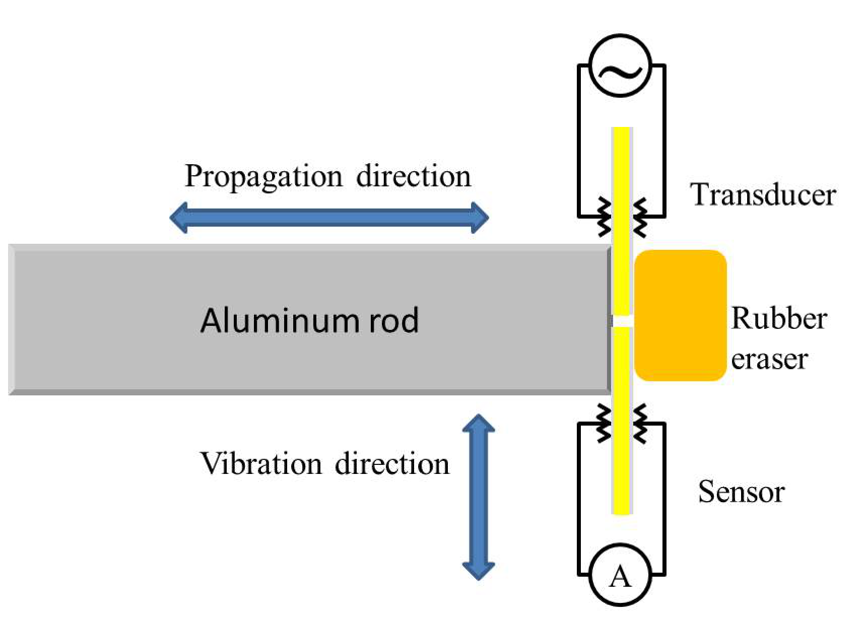
D.2 Use the steel tape measure to read the length of the aluminum rod. Please repeat the measurement several times and calculate the mean and the standard error.
While changing the frequency of the sound waves produced by the transducer, record the peak values monitored by the sensor. Draw a spectrum containing all measured resonant peaks, similar to that shown in Figure 12. [1,6 т.]
Instructions:
(1) Following steps 2 to 4 to arrange the experimental setup as illustrated in Figure 11. Note that the plastic box is specifically designed to accommodate the setup.
(2) Place the aluminum rod in the long trough of the plastic box, and use the eraser to press the PZT plates against one end of the aluminum rod, as illustrated in Figure 11. The two plates should not touch each other.
(3) Put the spring on the other end of the trough to gently push the rod against the PZT plates.
(4) Connect one PZT plate to the signal generator as the transducer. Connect the other PZT plate to the DMM as the sensor. Pay attention to the polarity when using the crocodile clips.
(5) The PZT plate is fragile and there is no extra supply.
(6) Use earplugs if you are annoyed by the high pitch sound.
(7) It is recommended that you sweep the frequency in the range between 0 and 40 kHz.
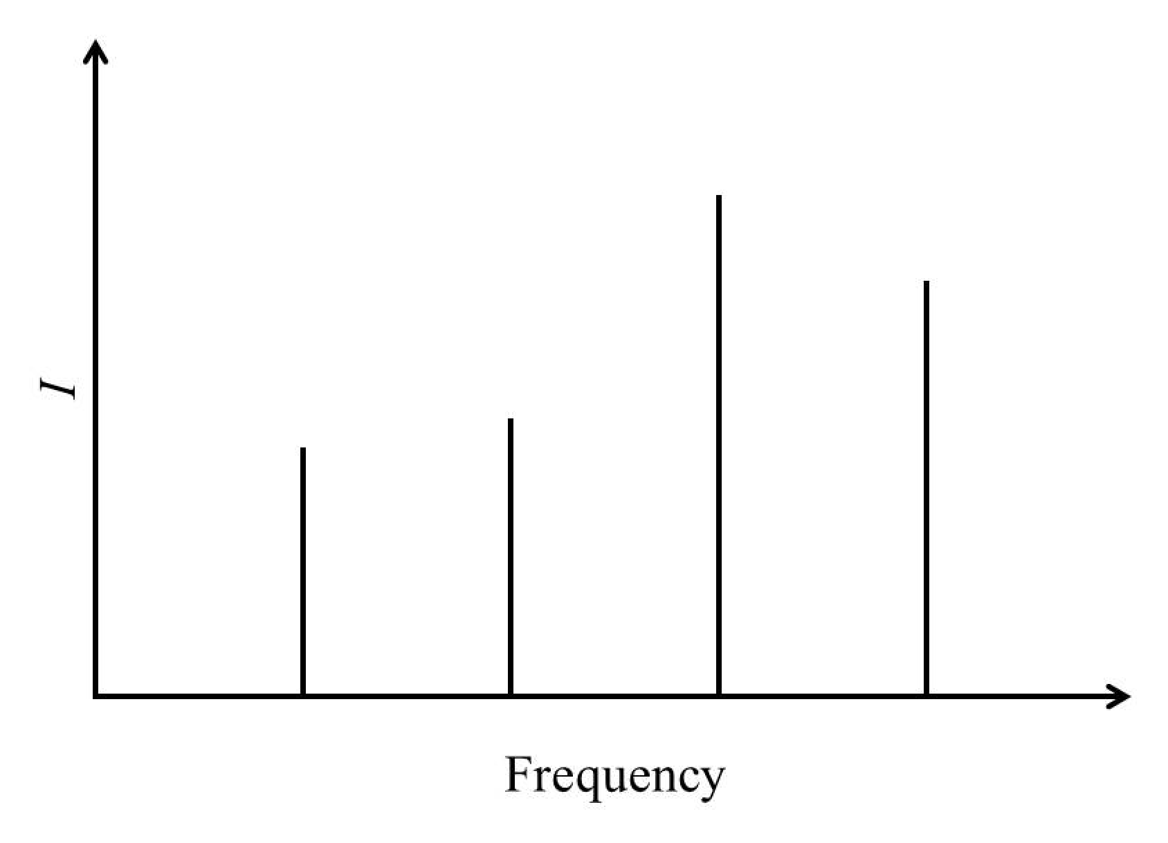
D.3 Identify the resonant peaks likely resulting from the transverse waves. Calculate the transverse wave velocity accordingly and carry out the error analysis.
Attention: there might be irrelevant peaks caused by imperfection of the experimental setup, e.g., imperfect free boundary condition. You need to make a judgement and ignore the irrelevant peaks during your analysis. [1,4 т.]
By changing the contact style between the PZT plates and the rod, we can also measure the longitudinal wave velocity in the rod. Attach the transducer and the sensor to the rod as illustrated in Figure 13. Vibration along the length direction of the transducer will propagate into the rod via compression, forming longitudinal waves.
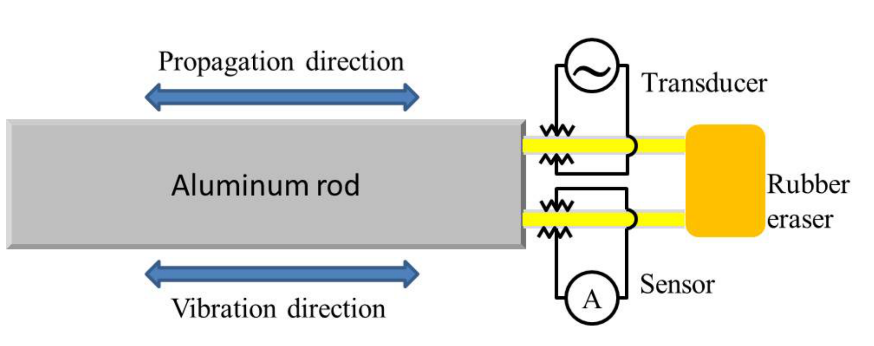
As discussed in Experiment B, although vibration along the length direction is dominant, vibrations along other directions also exist, which could produce sound waves in the rod and introduce extra resonant peaks in the spectrum as well. Note that vibrations along other directions only introduce transverse waves. Therefore the extra resonant peaks will not coincide with the peaks caused by the longitudinal standing waves.
D.4 While changing the frequency of the sound waves produced by the transducer, record the peak values monitored by the sensor. Draw a spectrum containing all measured resonant peaks, similar to that shown in Figure 12. [1,5 т.]
Instructions:
(1) Following steps 2 to 5 to arrange the experimental setup as illustrated in Figure 13. Note that the plastic box is specifically designed to accommodate the setup.
(2) Align two PZT plates in the two slim slots, respectively, on one end of the plastic box.
(3) With the long aluminum rod in the trough, use the eraser as a cushion to press the PZT plates against one end of the rod.
(4) Insert the spring on the other end to gently push the rod against the PZT plates.
(5) Connect one PZT plate to the signal generator as the transducer. Connect the other PZT plate to the DMM as the sensor. Note the polarity when using the crocodile clips.
(6) Attention: the style of contact between the PZT plates and the rod is crucial. Please have the edges of the PZT plates fully in touch with the side of the rod, so as to avoid point or partial contact.
(7) Attention: if you find too many resonant peaks in the spectrum, you can try to reduce the signal amplitude from the signal generator and/or slightly release the pressure between the PZT plates and the rod to reduce the production of transverse waves. You can also try to remove the spring on the other end if the contact between the PZT plates and the rod is still decent without the spring.
(8) It is recommended that you sweep the frequency between 0 and 40 kHz.
D.5 Compare with the result in D.2, identify the resonant peaks caused by the transverse waves. Select the resonant peaks resulting from the longitudinal waves and calculate the longitudinal wave velocity accordingly. Carry out the error analysis. [1,4 т.]
Experiment E — Application: locating a defect in an aluminum rod (2 т.)
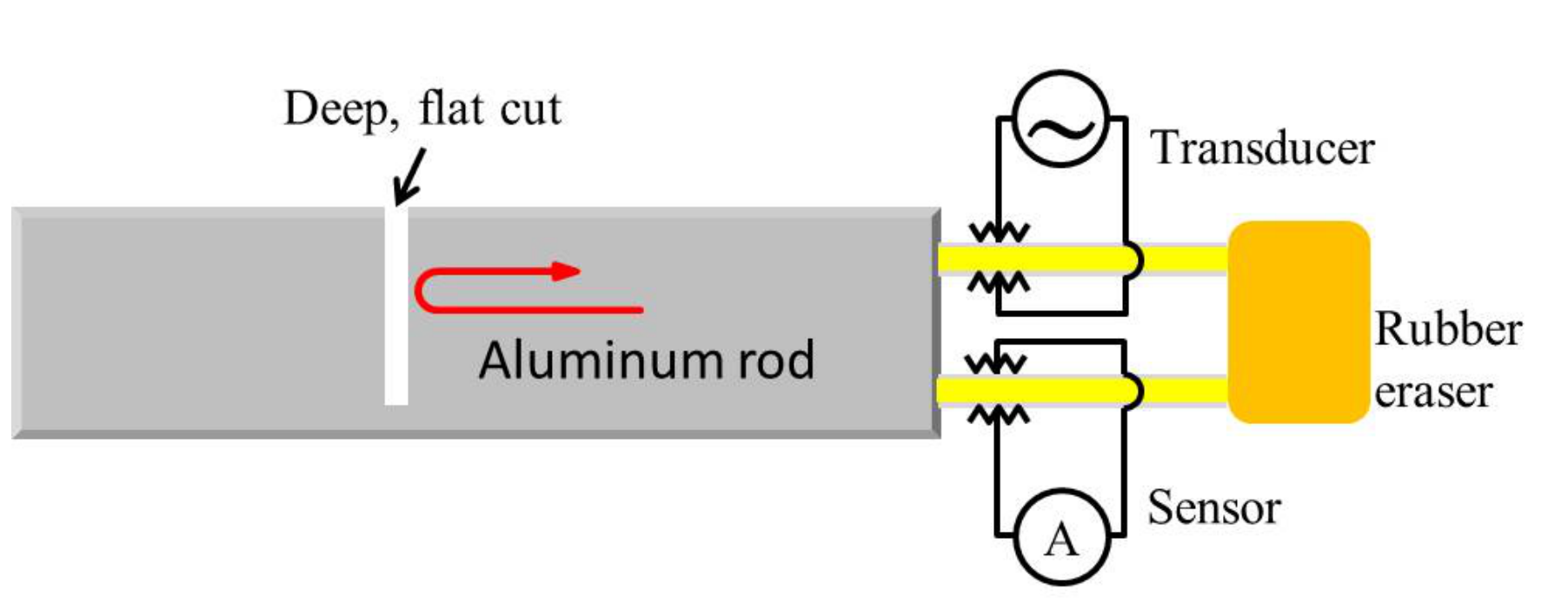
After knowing the longitudinal wave velocity from Experiment D, here we attempt to locate an artificially-engineered defect, a deep cut, along the long aluminum rod.
Sound waves through solid materials have been used to detect hidden cracks, voids, and other internal discontinuities in metals, composites, plastics, and ceramics. The industrial ultrasonic testing is done by repeatedly generating a several megahertz short pulse with an amplitude up to several hundred volts to drive the transducer, and then by amplifying the received signal to see if there is any reflection from a flaw. This is technically too complicated for our current setup. Instead, as a simple demonstration, we use the resonant method again to detect a deep, flat cut in the rod. Different from the case in Experiment D, sound waves will be bounced back at the spot of the deep cut instead of the far end of the rod. Therefore arrangement of the resonant peaks in the spectrum will be different from that in Experiment D, which can be the criterion for locating the spot of the deep cut.
The detection can be done using longitudinal waves.
E.1 While changing the frequency of the sound waves produced by the transducer, record the peak values monitored by the sensor. Draw a spectrum containing all measured resonant peaks, similar to that shown in Figure 12. [1,2 т.]
E.2 In the measured spectrum, identify the resonant peaks corresponding to the existence of the deep cut. Estimate the distance from the spot of the cut to the end of the rod that is in contact with the PZT plates. [0,8 т.]
Answer Sheets
Page1 of17

Page2 of17
Page3 of17

Page4 of17

Page5 of17

Page6 of17

Page7 of17

Page8 of17

Page9 of17

Page10 of17

Page11 of17

Page12 of17

Page13 of17

Page14 of17

Page15 of17

Page16 of17

Page17 of17

Решение
Marking Scheme — Experimental Competition, May 7, 2015, 08:30–13:30 hours. The cover says page 1 of 17. All native sample measurements, alternative calculations and scoring below are supplied by this marking scheme; the separate answer sheets remain unfilled.
A.1
Choose a PZT plate and use the Vernier caliper to measure its length , width and thickness . Use the electronic weighing scale to measure its mass . Use the DMM and the Kelvin clip to measure its capacitance (at ambient temperature).
Considering the slight non-uniformity in the dimensions of the PZT plate and the uncertainties of instrumental readings, repeat each measurement several times and then calculate the mean and the standard error.
| Measurement | (mm) | (mm) | (mm) | (g) | (nF) |
|---|---|---|---|---|---|
| 1 | 45.00 | 6.98 | 1.00 | 2.24 | 18.19 |
| 2 | 45.02 | 7.00 | 1.00 | 2.23 | 18.13 |
| 3 | 45.00 | 7.02 | 0.98 | 2.26 | 18.17 |
| 4 | 45.02 | 7.04 | 0.98 | 2.25 | 18.19 |
| 5 | 45.02 | 7.04 | 1.00 | 2.25 | 18.20 |
| 6 | 45.00 | 7.04 | 1.00 | 2.25 | 18.21 |
| Avg. |
Alternative:
If repeated measurement of dimension and mass gives the same result: , , , , and the six capacitances are 18.19,18.13,18.17,18.19,18.20,18.21 nF. The averages in the alternative table are mm, mm, mm, g and nF respectively.
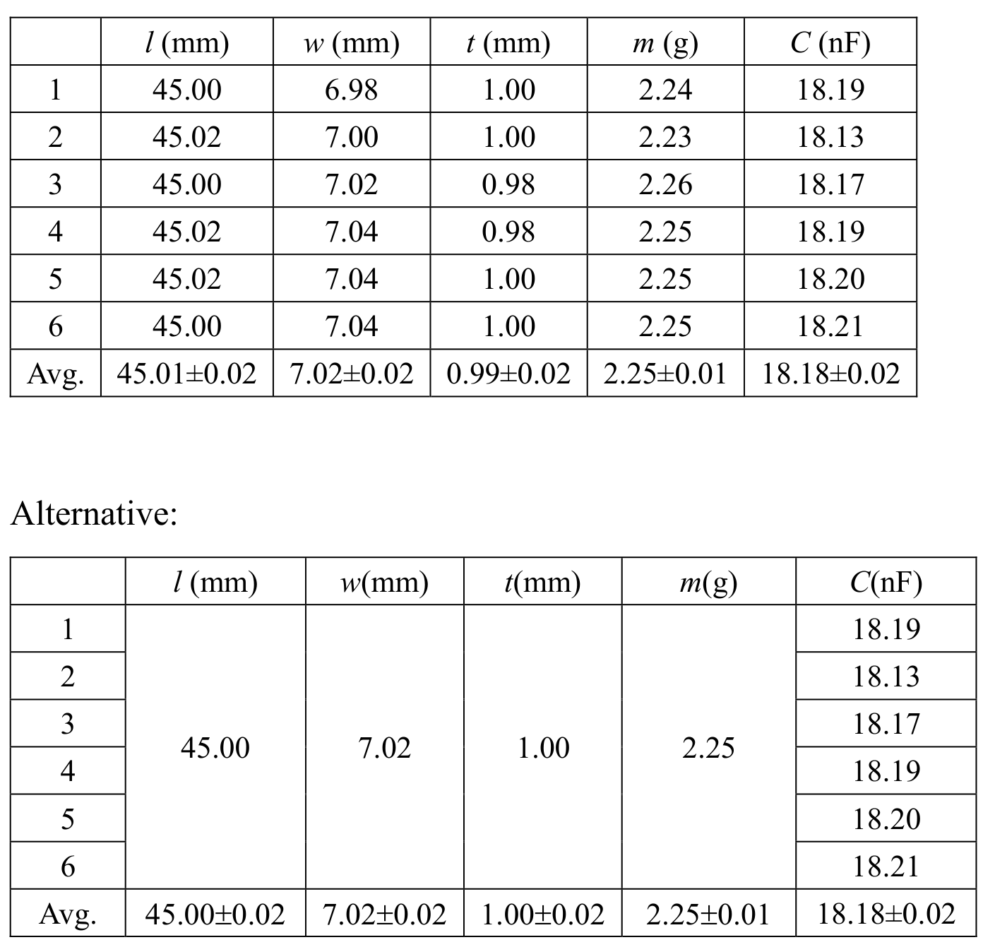
Total: 1.6. 0.2 data table. 0.2 units; −0.1 each unit missing. 0.3 standard error; −0.1 each error missing. 0.3 correct number of significant figures; −0.1 each wrong significant figure. 0.3 correct reading of Vernier caliper. 0.2 right value of : 0.2 for 17.30–19.10 nF; 0.1 for 16.40–17.30 nF or19.10–20.00 nF;0 otherwise. 0.2 repeated measurement of capacitance:0.2 repeat≥6times;0.1 repeat≥3times;0 otherwise.
A.2
Now calculate the density and the relative permittivity of the PZT plate. Based on standard errors obtained from A.1, carry out the error analysis to estimate the uncertainties of and (vacuum permittivity ).
Alternative: calculate each time:7.13,7.08,7.30,7.24,7.10,7.10,
Or
Total:1.4. 0.1 unit of .0.2 right value of :0.2 for6.85–7.55;0.1 for6.50–6.85 or7.55–7.90;0 otherwise.0.2 expression.0.2 right value of :0.2 for0.05–0.30;0.1 for0.01–0.05 or0.30–0.50;0 otherwise. The same criteria for .0.2 right value of :0.2 for6.10–6.80;0.1 for5.75–6.10 or6.80–7.15;0 otherwise.0.2 right value of :0.2 for0.05–0.30;0.1 for0.01–0.05 or0.30–0.50;0 otherwise.
Alternative:0.2 ;0.1 unit of ;0.1 expression;0.1 right value of :0.1 for0.01–0.40,0 otherwise.0.2 data points:0.2 measure≥6times;0.1 for3–5times;0 otherwise. The same criteria for .
B.1
Derive the expressions for the resonant frequency and the antiresonant frequency of the equivalent circuit.
The impedance of the capacitance , and inductance are
Respectively. Assume the total impedance of the equivalent circuit is , then we have
Resonance condition:
Antiresonance condition:
Total:1.0. 0.1 impedance;0.1 impedance;0.1 impedance;0.3 total impedance;0.2 resonant frequency;0.2 antiresonant frequency.
B.2
Measure the AC current through the PZT plate as a function of the signal frequency . Draw the - curve and find the resonant frequency and the antiresonant frequency . Calculate the piezoelectric coefficient accordingly.
| Freq (kHz) | (mA) | Freq (kHz) | (mA) | Freq (kHz) | (mA) | Freq (kHz) | (mA) |
|---|---|---|---|---|---|---|---|
| 2 | 0.58 | 30.5 | 20.86 | 32.4 | 4.82 | 34.3 | 1.18 |
| 4 | 1.13 | 30.6 | 21.28 | 32.5 | 4.06 | 34.0 | 1.37 |
| 6 | 1.68 | 30.7 | 21.50 | 32.6 | 3.37 | 34.5 | 1.52 |
| 8 | 2.21 | 30.8 | 21.47 | 32.7 | 2.76 | 34.6 | 1.67 |
| 10 | 2.75 | 30.9 | 21.13 | 32.8 | 2.20 | 34.7 | 1.82 |
| 12 | 3.29 | 31.0 | 20.51 | 32.9 | 1.73 | 34.8 | 1.96 |
| 14 | 3.85 | 31.1 | 19.64 | 33.0 | 1.29 | 34.9 | 2.10 |
| 16 | 4.42 | 31.2 | 18.55 | 33.1 | 0.94 | 35 | 2.23 |
| 18 | 5.03 | 31.3 | 17.35 | 33.2 | 0.66 | 36 | 3.35 |
| 20 | 5.69 | 31.4 | 16.06 | 33.3 | 0.47 | 37 | 4.18 |
| 22 | 6.46 | 31.5 | 14.73 | 33.4 | 0.36 | 38 | 4.82 |
| 24 | 7.39 | 31.6 | 13.40 | 33.5 | 0.31 | 39 | 5.34 |
| 26 | 8.72 | 31.7 | 12.10 | 33.6 | 0.33 | 40 | 5.78 |
| 28 | 11.05 | 31.8 | 10.85 | 33.7 | 0.38 | ||
| 30 | 17.69 | 31.9 | 9.65 | 33.8 | 0.48 | ||
| 30.1 | 18.34 | 32.0 | 8.55 | 33.9 | 0.60 | ||
| 30.2 | 18.99 | 32.1 | 7.50 | 34.0 | 0.74 | ||
| 30.3 | 19.66 | 32.2 | 6.52 | 34.1 | 0.89 | ||
| 30.4 | 20.29 | 32.3 | 5.63 | 34.2 | 1.04 |
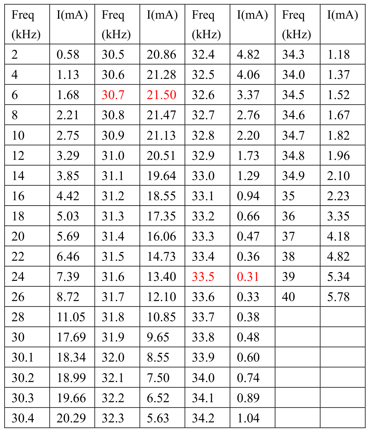
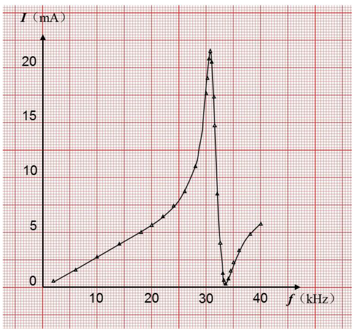
Total:3.5. 0.2 data table;0.2 units;0.3 significant figures;0.3 ≥10data points;0.3 ;0.3 ;0.3 0.1kHz frequency resolution near and .0.5 figure:0.1 data points,0.1 units,0.1 axis label,0.1 axis ticks label,0.1 smooth curve.0.1 unit of .1.0 right value of :1.0 for4.20–4.70;0.5 for3.95–4.20 or4.70–4.95;0 otherwise.
Source note: the sample table prints34.0kHz between34.3 and34.5; the retained native table shows this literal value and its red resonant/antiresonant highlights.
C.1
Now measure the capacitance of the PZT plate at various temperatures and record the data.
| (°C) | 17.0 | 30.0 | 40.0 | 50.0 | 60.0 | 70.0 | 80.0 |
|---|---|---|---|---|---|---|---|
| (nF) | 16.80 | 18.25 | 19.77 | 21.08 | 23.07 | 25.60 | 27.80 |
| (nF⁻¹) | 0.0595 | 0.0548 | 0.0506 | 0.0474 | 0.0433 | 0.0391 | 0.0360 |

Total:1.5. 0.2 data table;0.2 units;0.2 significant figures;0.4 data points:0.4 ≥6data points,0.2 for4–5data points,0 otherwise.0.5 temperature range:0.5 from room temperature to≥80°C;0.3 temperature range35–50°C;0.1 temperature range20–35°C;0 otherwise.
C.2
Analyze the data, draw a proper plot and calculate the Curie temperature accordingly.
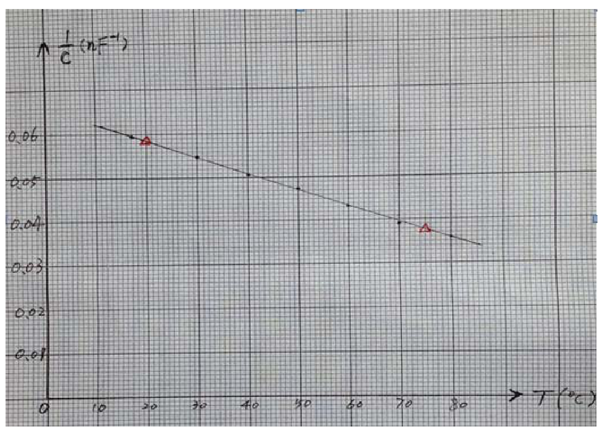
From the straight line choose two points , to calculate the slope
We can get the linear function
Let , then we can get the Curie temperature
Alternative method: extent the straight line to intercept with the x axis to get the Curie temperature.
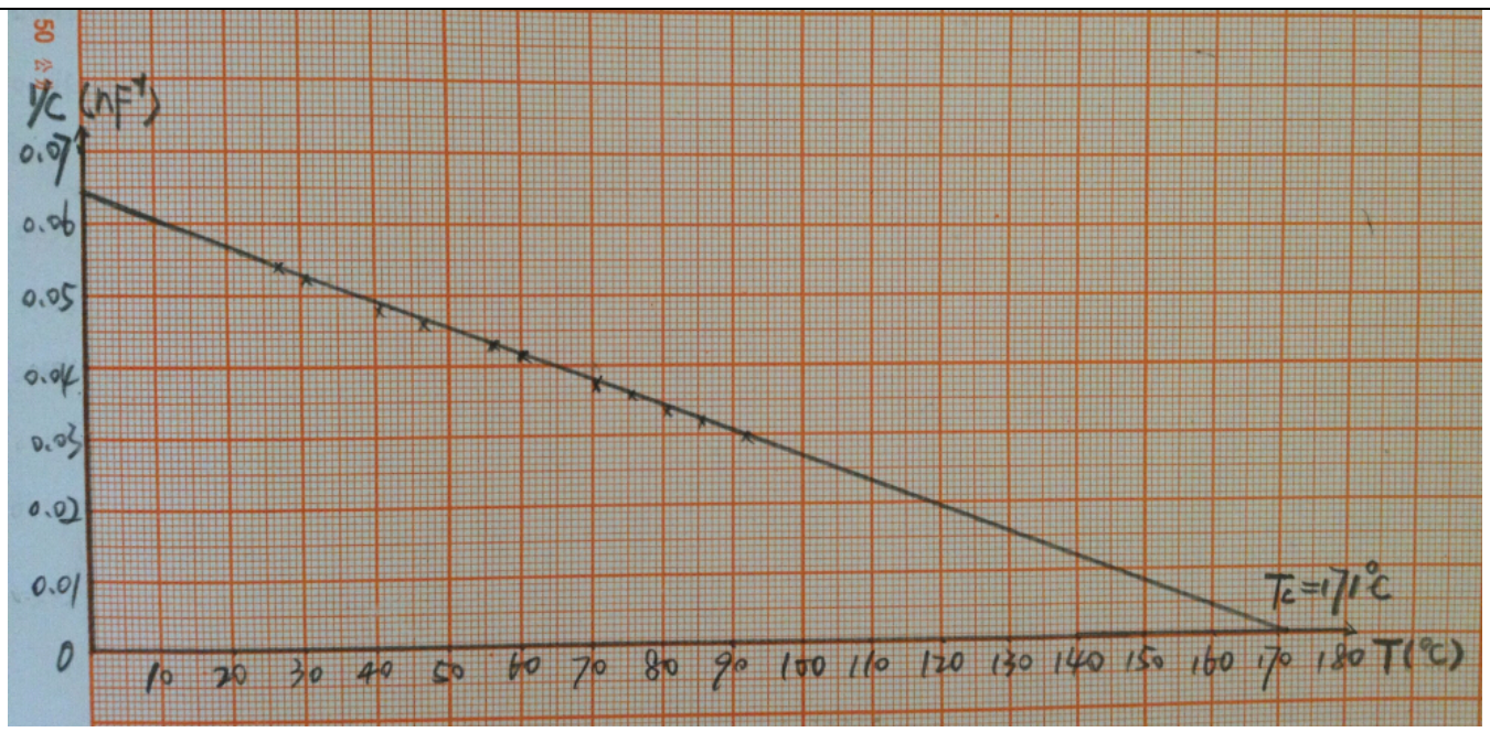
Total:2.5. 0.1 axis label;0.1 axis unit;0.1 axis tick label;0.3 Choice of Scale (to cover70%or more space on graph sheet);0.2 data marker;0.2 straight line;0.2 proper choice of ;0.2 slope;0.2 significant figures;0.2 linear function;0.1 unit of ;0.6 right value of :0.6 for160–180,0.3 for150–160 or180–190;0 otherwise. Note: other reasonable method that yields correct result is acceptable.
Alternative:1.0 at most;0.3 extent straight line to intercept with x axis;0.1 unit of ;0.6 right value of .
Source note: the analytic answer prints174°C, while the alternative native graph marks176°C. Both are retained as printed.
D.1
Assume that the length of the aluminum rod is and the wave velocity is . Under the free boundary condition, derive the equation for the frequencies of the standing (resonant) waves along the long rod. Then derive the equation for the wave velocity from .
Consider the aluminum rod as a one dimensional long string with free Boundary condition, then the standing wave condition is
According to
The standing wave frequencies are
Continually changing the vibration frequency, we can find out a series of standing wave frequencies and calculate the average distance between two peaks , we have
Total:0.6. 0.2 eqn.(1);0.1 eqn.(2);0.1 eqn.(3);0.2 eqn.(4). Note: express in terms of instead of is also acceptable.
D.2
Use the steel tape measure to read the length of the aluminum rod. Please repeat the measurement several times and calculate the mean and the standard error.
While changing the frequency of the sound waves produced by the transducer, record the peak values monitored by the sensor. Draw a spectrum containing all measured resonant peaks, similar to that shown in Figure 12.
| Measurement | 1 | 2 | 3 | 4 | 5 | 6 | Avg |
|---|---|---|---|---|---|---|---|
| (cm) | 49.93 | 49.98 | 50.00 | 50.02 | 50.05 | 50.03 |
| (kHz) | 6.37 | 8.81 | 11.81 | 14.70 | 17.54 | 20.45 | 23.44 |
|---|---|---|---|---|---|---|---|
| (μA) | 16.5 | 42.6 | 144.0 | 249.5 | 336.9 | 247.7 | 358.4 |
| (kHz) | 26.40 | 29.47 | 31.14 | 32.35 | 35.22 | 38.76 | 40.13 |
| (μA) | 296.2 | 429.9 | 109.2 | 907 | 671 | 446.8 | 479 |
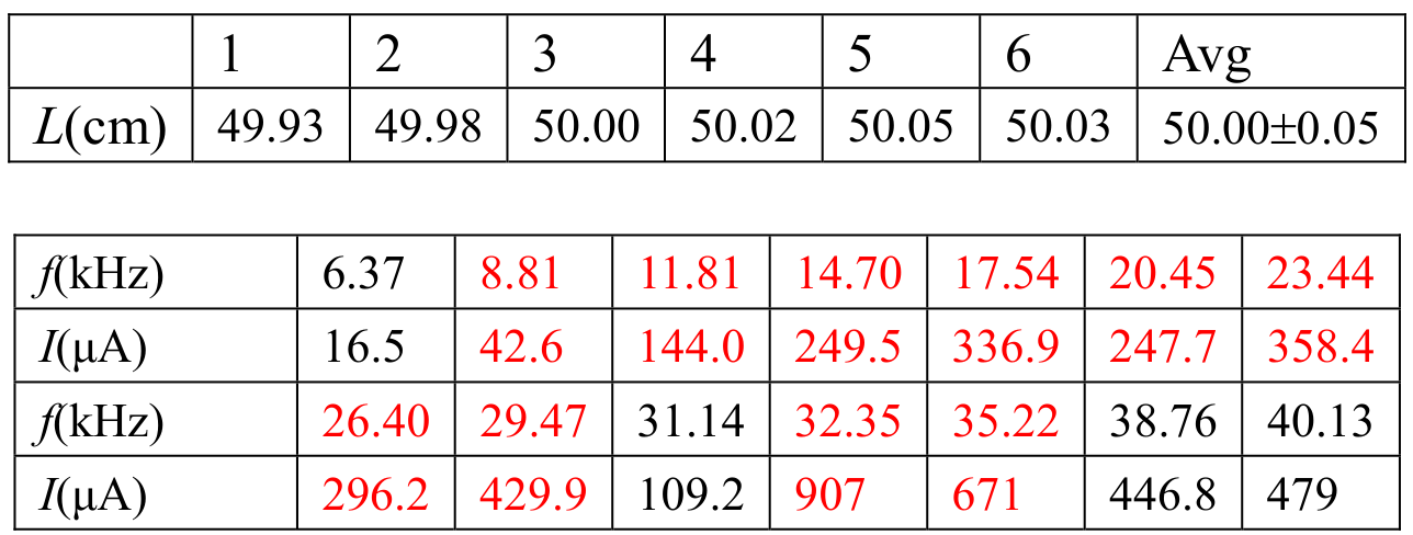
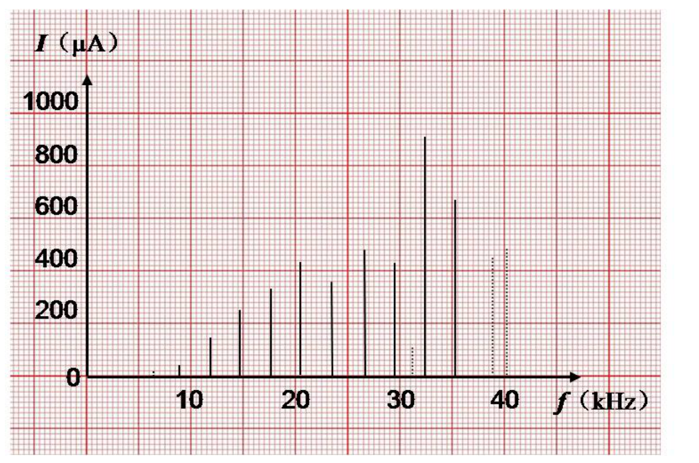
Total:1.6. 0.1 multi measurement;0.1 value of ;0.1 error of ;0.1 units;0.1 significant figures;0.1 ≥10data points;0.4 standing wave peaks resulting from the transverse waves:0.4 ≥6peaks,0.2 for3–5peaks,0 otherwise;0.3 frequency resolution0.01kHz;0.1 at least one miscellaneous peak;0.2 spectrum containing all measured peaks.
D.3
Identify the resonant peaks likely resulting from the transverse waves. Calculate the transverse wave velocity accordingly and carry out the error analysis.
Attention: there might be irrelevant peaks caused by imperfection of the experimental setup, e.g., imperfect free boundary condition. You need to make a judgement and ignore the irrelevant peaks during your analysis.
| (kHz) | |
|---|---|
| 1 | 8.81 |
| 2 | 11.81 |
| 3 | 14.70 |
| 4 | 17.54 |
| 5 | 20.45 |
| 6 | 23.44 |
| 7 | 26.40 |
| 8 | 29.47 |
| 9 | 32.35 |
| 10 | 35.22 |
(kHz): , , , , , . The printed values are0.08,0.12,0.06,0.10,0.06kHz, and the final table entry is .
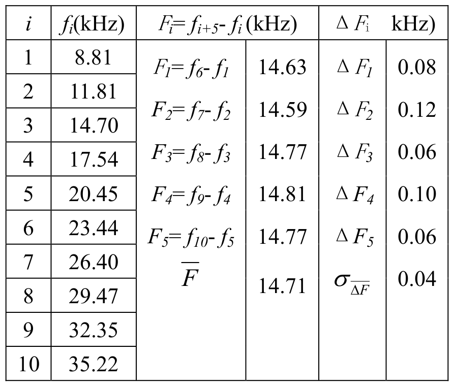
Total:1.4. 0.3 successive difference method. Note: other reasonable method that yields correct result is acceptable.0.1 data table;0.1 significant figures;0.1 unit;0.6 right value of transverse wave velocity:0.6 for2.80–3.10km/s,0.2 for2.65–2.80km/s or3.10–3.25km/s,0 otherwise;0.2 right value of :0.2 for0.01–0.15km/s,0.1 for0.15–0.30km/s,0 otherwise.
D.4
While changing the frequency of the sound waves produced by the transducer, record the peak values monitored by the sensor. Draw a spectrum containing all measured resonant peaks, similar to that shown in Figure 12.
| (kHz) | 5.18 | 8.90 | 10.50 | 14.53 | 15.53 | 20.63 | 23.39 | 24.68 | 25.67 |
|---|---|---|---|---|---|---|---|---|---|
| (μA) | 15.5 | 52.7 | 216.2 | 103.6 | 353.3 | 555 | 156.4 | 45.8 | 1328 |
| (kHz) | 26.44 | 29.40 | 30.64 | 32.33 | 35.20 | 35.55 | 37.81 | 38.74 | 40.26 |
| (μA) | 414.5 | 848 | 1940 | 1593 | 2589 | 2331 | 1043 | 118.8 | 450 |
| (kHz) | 40.79 | 41.53 | |||||||
| (μA) | 194.5 | 32.7 |
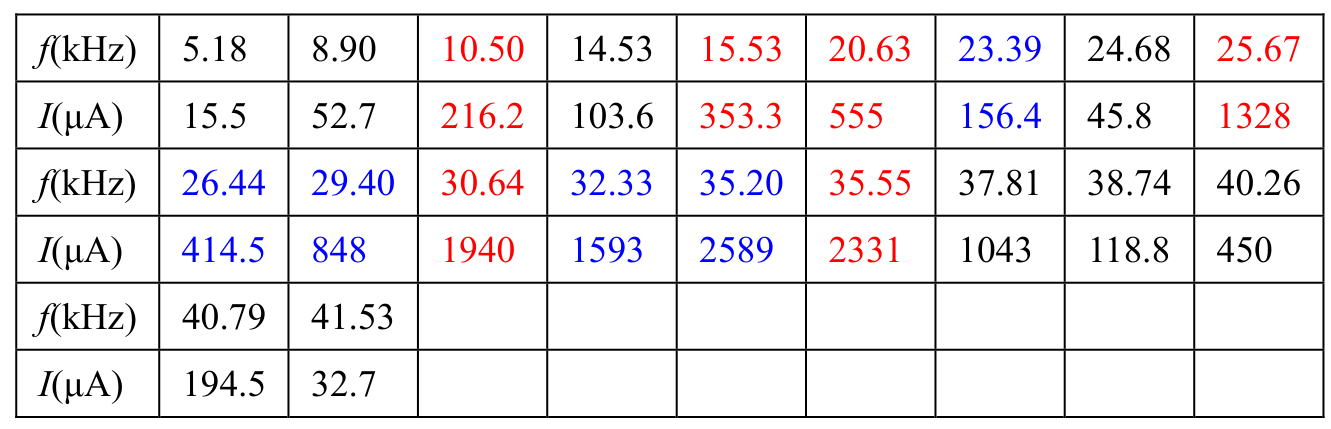
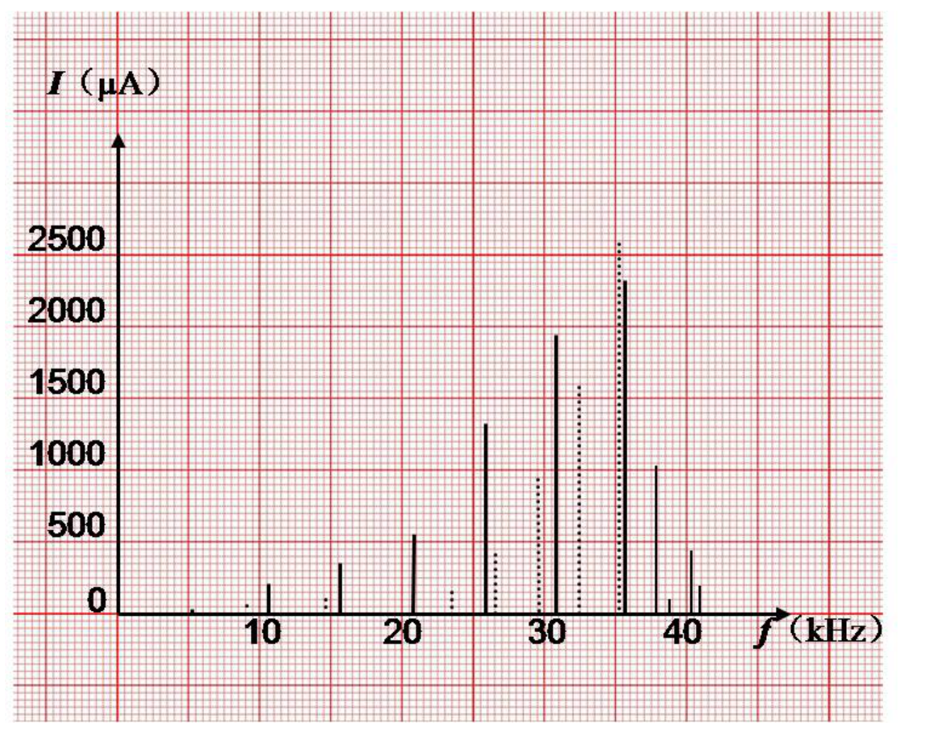
Total:1.5. 0.1 unit;0.1 significant figures;0.1 >10data points;0.4 standing wave peaks resulting from the longitudinal waves:0.4 ≥6peaks,0.2 for3–5peaks,0 otherwise;0.2 standing wave peaks resulting from the transverse waves:0.2 ≥4peaks,0.1 for2–3peaks,0 otherwise;0.3 frequency resolution0.01kHz;0.1 at least one miscellaneous peak;0.2 spectrum containing all measured peaks.
D.5
Compare with the result in D.2, identify the resonant peaks caused by the transverse waves. Select the resonant peaks resulting from the longitudinal waves and calculate the longitudinal wave velocity accordingly. Carry out the error analysis.
Selected longitudinal values (kHz):“10 50”,15.53,20.63,25.67,30.64,35.55.
(kHz): , , , . The printed values are0.10,0.04,0.15kHz, and the final table entry is .
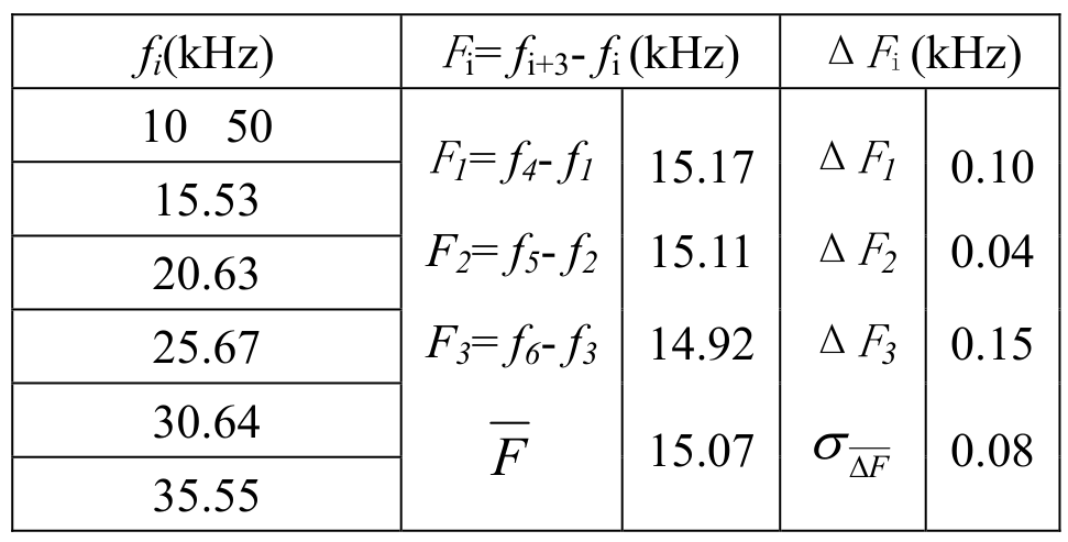
Thus the longitudinal wave velocity is given by
Total:1.4. 0.3 successive difference method. Note: other reasonable method that yields correct result is acceptable.0.1 data table;0.1 significant figures;0.1 units;0.6 right value of longitudinal wave velocity:0.6 for4.70–5.20km/s,0.3 for4.50–4.70km/s or5.20–5.40km/s,0 otherwise;0.2 right value of :0.2 for0.01–0.20km/s,0.1 for0.20–0.40km/s,0 otherwise.
Source note: both native D.3 and D.5 uncertainty formulas print ; that notation has been preserved.
Source note: the first frequency in this key table is printed “10 50” with no visible decimal; the preceding D.4 table prints 10.50 kHz. Both original displays are preserved.
E.1
While changing the frequency of the sound waves produced by the transducer, record the peak values monitored by the sensor. Draw a spectrum containing all measured resonant peaks, similar to that shown in Figure 12.
| (kHz) | 5.06 | 8.01 | 8.85 | 10.09 | 15.05 | 15.14 | 17.15 | 20.11 |
|---|---|---|---|---|---|---|---|---|
| (μA) | 9.1 | 6.1 | 66.0 | 43.8 | 34.9 | 105.2 | 358.9 | 57.2 |
| (kHz) | 24.95 | 25.17 | 30.27 | 33.37 | 35.27 | 39.23 | 40.82 | 41.05 |
| (μA) | 150.9 | 751 | 441 | 432.7 | 430.1 | 241.9 | 242.4 | 57.7 |
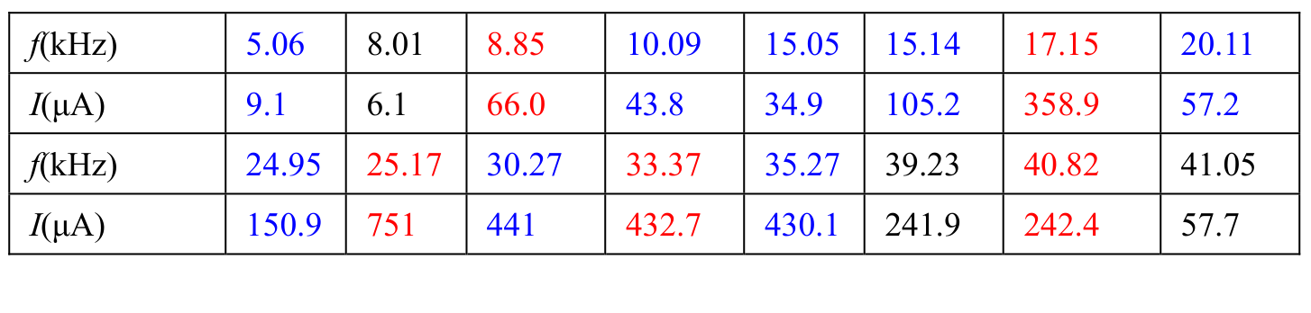
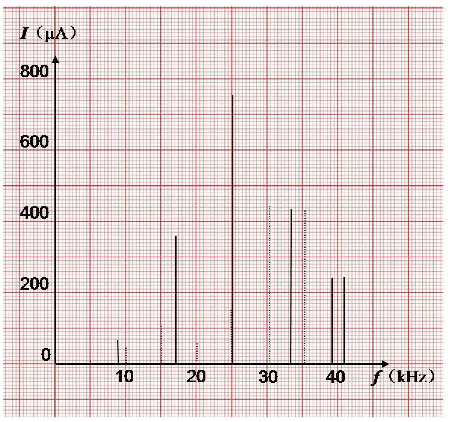
Total:1.2. 0.1 unit;0.1 significant figures;0.1 >10data points;0.2 resonant peaks of the longitudinal waves corresponding to the cut:0.2 ≥4peaks,0.1 for2–3peaks,0 otherwise;0.1 at least2resonant peaks of the transverse waves;0.3 frequency resolution0.01kHz;0.1 at least one miscellaneous peak;0.2 spectrum containing all measured peaks.
E.2
In the measured spectrum, identify the resonant peaks corresponding to the existence of the deep cut. Estimate the distance from the spot of the cut to the end of the rod that is in contact with the PZT plates.
| (kHz) | 8.85 | 17.15 | 25.17 | 33.37 | 40.82 |
|---|---|---|---|---|---|
| (μA) | 66.0 | 358.9 | 751 | 432.7 | 242.4 |
(kHz):16.32,16.22,15.65. The table prints .
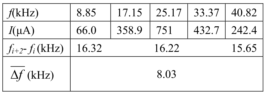
Total:0.8. 0.1 significant figures;0.1 units;0.6 right value of distance:0.6 for0.28–0.32m,0.3 for0.26–0.28m or0.32–0.34m,0 otherwise.
Source note: the native table gives8.03kHz whereas the following equation gives8.11kHz; its printed final distance is0.307m. All three values are retained without supplying a replacement official result. The marking scheme also contains measured frequencies above the question's recommended0–40kHz sweep range.
Теми и трудност
Оценена трудност: 4/5.
Вълни и звук · Електричество · Механика · Звук и акустика · Кондензатори и диелектрици · Резонанс и затихване
Предпоставки: Гимназиална подготовка, Разширена олимпиадна подготовка
Оригинал в Архива: exp.pdf · официални решения: exp_sol.pdf · допълнителни данни: exp_anssheet.pdf