APhO 2015, Теория — Задача 2. How are aurora ignited by the solar wind?
16th ASIAN PHYSICS OLYMPIAD 2015 — Question 2 · 3 май 2015 г.
Условие
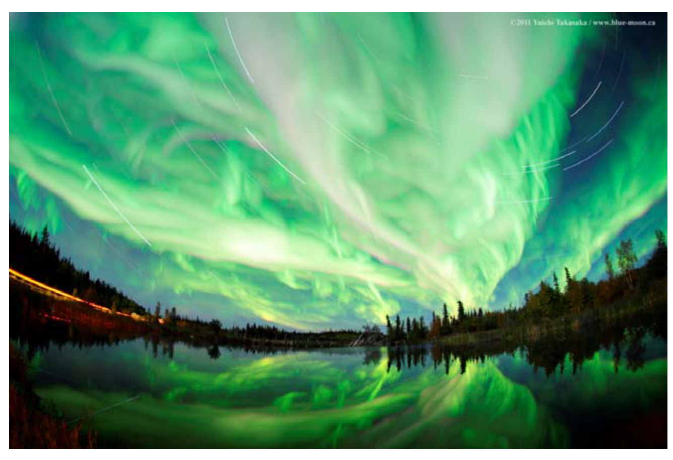
The following questions are designed to guide you to find the answer one step by one step.
Background information of the interaction between the solar wind and the Earth's magnetic field
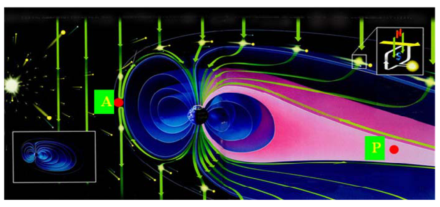
It is well known that the Earth has a substantial magnetic field. The field lines defining the structure of the Earth's magnetic field is similar to that of a simple bar magnet, as shown in Figure 2. The Earth's magnetic field is disturbed by the solar wind, which is a high-speed stream of hot plasma. (The plasma is the quasi-neutral ionized gas.) The plasma blows outward from the Sun and varies in intensity with the amount of surface activity on the Sun. The solar wind compresses the Earth's magnetic field. On the other hand, the Earth's magnetic field shields the Earth from much of the solar wind. When the solar wind encounters the Earth's magnetic field, it is deflected like water around the bow of a ship, as illustrated in Figure 3.
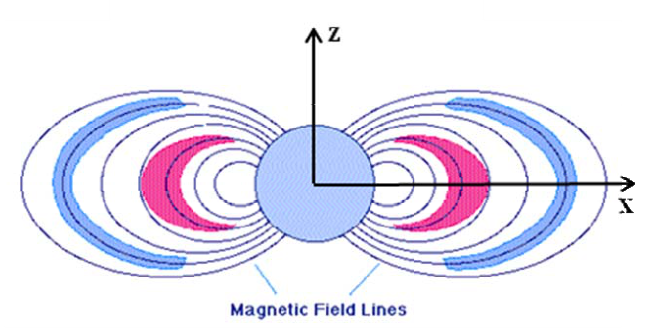
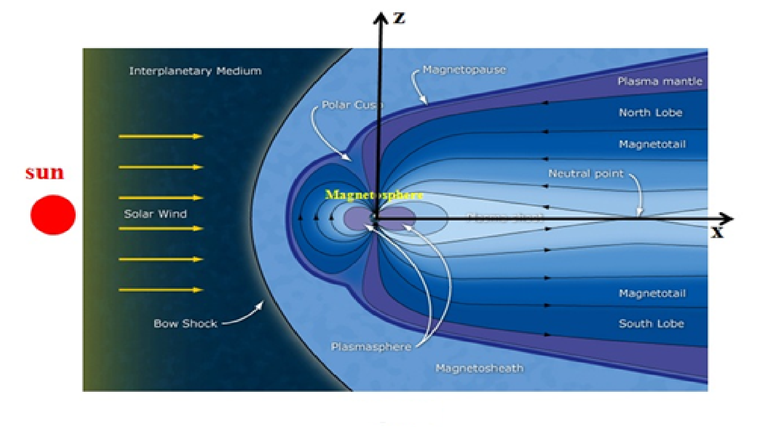
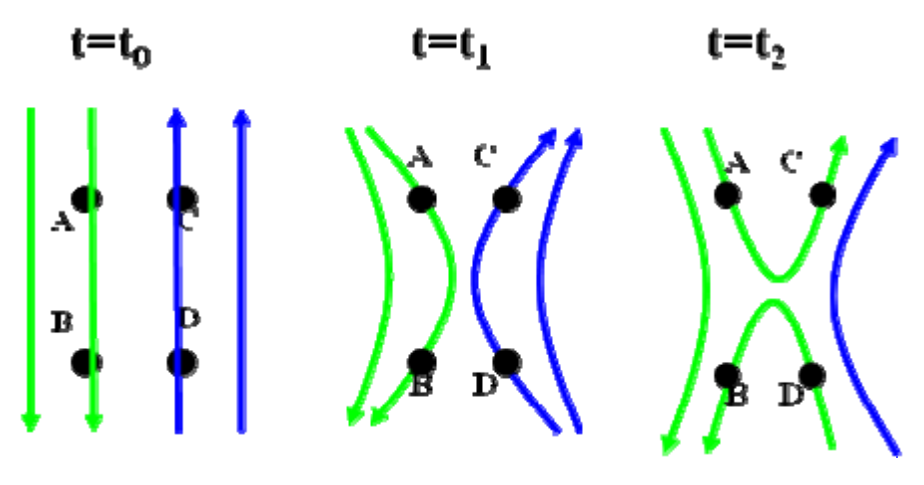
The curved surface at which the solar wind is first deflected is called the bow shock. The corresponding region behind the bow shock and front of the Earth's magnetic field is called the magnetosheath. The region surrounded by the solar wind is called the magnetosphere. The Earth's magnetic field largely prevents the solar wind from entering the magnetosphere. The contact region between the solar wind and the Earth's magnetic field is named the magnetopause. The location of the magnetopause is mainly determined by the intensity and the magnetic field direction of the solar wind. When the magnetic field in the solar wind is antiparallel to the Earth's magnetic field, magnetic reconnection as shown in Figure 4 takes place at the dayside magnetopause, which allows some charged particles of the solar wind in the region "A" to move into the magnetotail "P" on the night side as illustrated in Figure 5. A powerful solar wind can push the dayside magnetopause to very close to the Earth, which could cause a high-orbit satellite (such as a geosynchronous satellite) to be fully exposed to the solar wind. The energetic particles in the solar wind could damage high-tech electronic components in a satellite. Therefore, it is important to study the motion of charged particles in magnetic fields, which will give an answer of the aurora generation and could help us to understand the mechanism of the interaction between the solar wind and the Earth's magnetic field.
Numerical values of physical constants and the Earth's dipole magnetic field:
Speed of light in vacuum: ;
Permittivity in vacuum: ;
Permeability in vacuum: ;
Charge of a proton: ;
Mass of an electron: ;
Mass of a proton: ;
Boltzmann's constant: ;
Gravitational acceleration: ;
Planck’s constant:
Earth's radius .
The Earth's dipole magnetic field can be expressed as
where , , and are the unit vectors in the , , directions, respectively.
Questions:
(a) (3 т.)
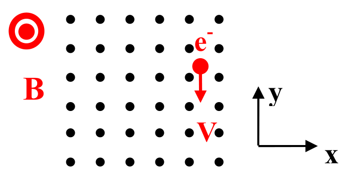
(i) Before we study the motion of a charged particle in the Earth's dipole magnetic field, we first consider the motion of an electron in a uniform magnetic field . When the initial electron velocity is perpendicular to the uniform magnetic field as shown in Figure 6, please calculate the electron trajectory. The electron is initially located at (x,y,z)=(0,0,0). [1 т.]
(ii) Please determine the electric current of the electron motion and calculate the magnetic moment , where is the area of the electron circular orbit and the direction of is determined by the right-hand rule of the electric current. [1 т.]
(iii) If the initial electron velocity is not perpendicular to the uniform magnetic field, i.e, the angle between and is , please give the screw pitch (the distance along the z-axis between successive orbits) of the electron trajectory. [1 т.]
(b) (4 т.)
In the uniform background magnetic field as shown in Figure 6, the plasma density is nonuniform in x. For simplicity, we assume that the temperature and the distribution of the ions and electrons are the same. Thus, the plasma pressure can be expressed as
Where B, T, k, , and are positive constants, and are the number densities of the ions and electrons.
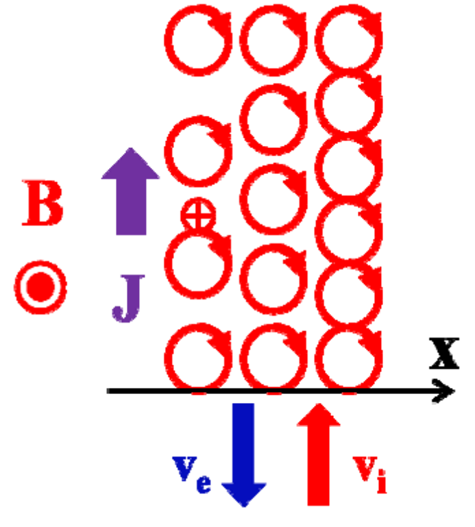
(i) Please explain the generation mechanism of the electric current by a schematic drawing. [2 т.]
(ii) If both the ions and electrons have a Maxwellian distribution, the ion distribution is
please calculate the constant β in the magnetization , where the magnetization M is the magnetic moment per unit volume. (Hint: We have and .) [2 т.]
(c) (1 т.)
Now let's go back to the Earth's dipole magnetic field. Please apply the result from Question(b) to calculate the ratio of the diamagnetic field and the Earth's dipole magnetic field in Equation (1) at the position (=10R,=0, =1 R). The plasma pressure is assumed to be , where and . The magnetic field around this position is also assumed to be uniform. Be aware of the difference in the coordinate systems in Questions (b) and (c). (Hint: The diamagnetic field is given by .)
(d) (4 т.)
From Figures 2, 3, and 5, it can be clearly seen that the Earth's magnetic field strength along a magnetic field line is the largest at the poles and the smallest in the equatorial plane. Since the Earth's dipole magnetic field is axially symmetric and slowly varying along a magnetic field line, it can for simplicity be treated as a magnetic-mirror field as shown in Figure 7. The magnetic field strength along a magnetic field line is the smallest () at the point "P" and the largest () at the points "P" and "P". An electron with an initial velocity is located at the point "P" and drifts towards the point "P". The angle between the initial velocity and the magnetic field at the point "P" is . For the magnetic-mirror field (with ), we can assume , where is the spatial derivative of along a magnetic field line. Since there is no evidence of the existence of magnetic monopoles, we have , where is the gyro-average of and is the electron gyroradius.
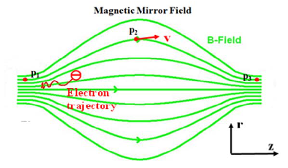
(i) Please give the gyro-averaged magnetic-field force along the magnetic field lines on an electron and show that the magnetic moment is a motion constant, i.e., , based on the law of the total kinetic energy conservation. [3 т.]
(ii) Based on the motion constant of magnetic moment, please determine what the condition should be satisfied for the angle between the initial electron velocity and the magnetic field at the point "P" if an electron will not escape from the magnetic mirror field. [1 т.]
(e) (1 т.)
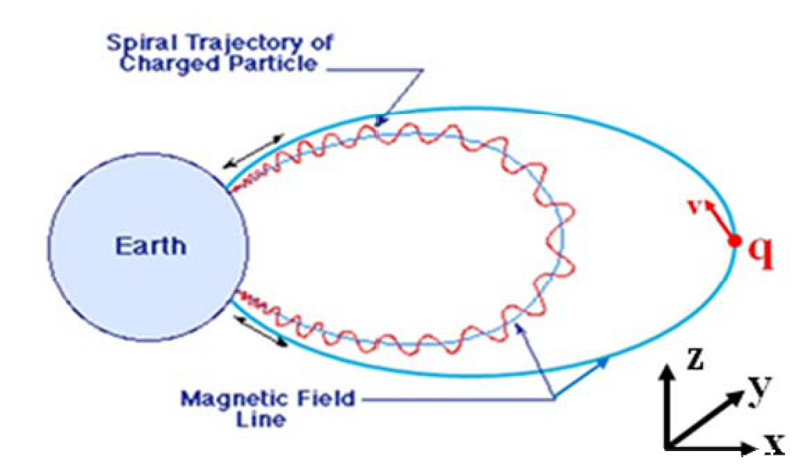
Earth's dipole magnetic field lines (blue lines) are shown in Figure 8. The spiral trajectory of a charged particle (red curve) is assumed to be confined in the =0 plane since the gradient and the curvature of the magnetic field can be ignored. If a charged particle with the mass , charge , and velocity is initially located at the equatorial position [=6R, =0, =0] and the angle between the electron velocity and the magnetic field is initially, please determine what the condition should be satisfied for if the charged particle arrives below 200km of its altitude at the latitude .
(f) (5 т.)
As shown in Figure 5, when magnetic reconnection takes place at the dayside magnetopause, reconnected magnetic field lines drift towards the nightside region because the solar wind flows tailward. Thus, some solar wind electrons in the region "A" also move towards the magnetotail in the region "P". After the electrons arrive in the region "P", some electrons can be accelerated to around 1keV. If energetic electrons drift down to the thermosphere (The altitude of the thermosphere is about 85km-800km.), energetic electrons can collide with the neutral atoms, which could cause the neutral atoms to jump into excited states. A photon is emitted when the higher excited state of a neutral atom returns to its lower excited state or ground state. Splendid aurora (Figure 1) is generated in the aurora oval due to photons with different wavelengths. It is found that the aurora is mainly resulted from photons emitted by oxygen atoms. The energy levels in the first and second excited states relative to the ground state are 1.96eV and 4.17eV, respectively. The lifetimes of the two excited states of an oxygen atom are 110s and 0.8s as shown in Figure 9.
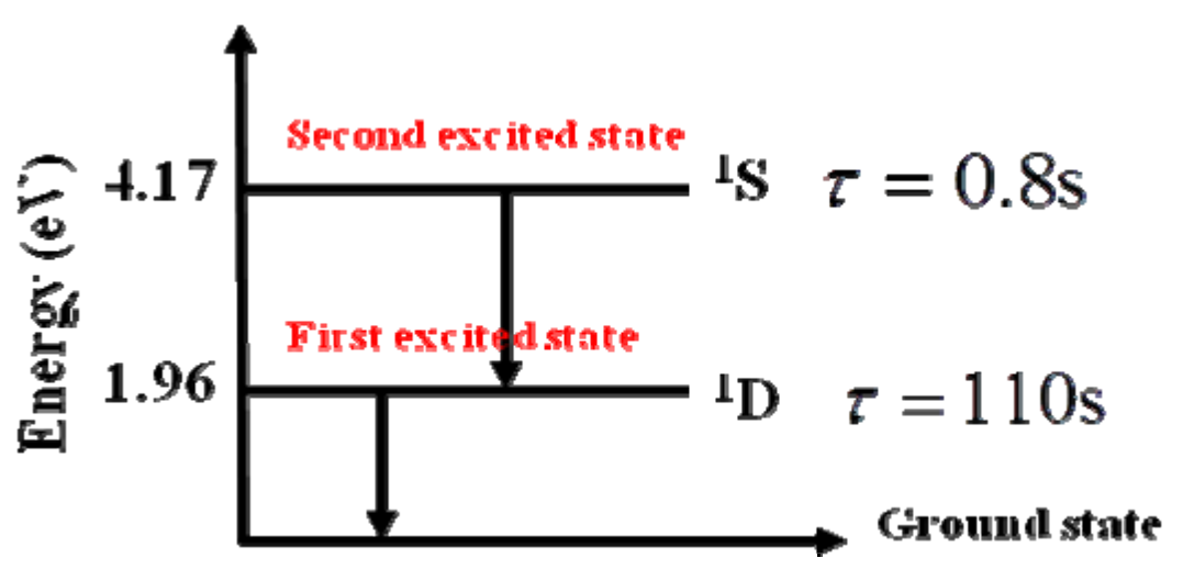
(i) Please give the atmospheric density as a function of the altitude and the ratio of the oxygen density at the altitudes H=160km and H=220km. For simplicity, we assume that the atmospheric temperature is independent of the altitude and the air is an ideal gas.
(, where and are the atmospheric density and pressure at sea level.) [2 т.]
(ii) Please give the colors of auroras at the altitudes H=160km and H=220km. (Hint: The dependence of the collision frequency of atmospheric molecules on the atmospheric density is , where is the collision frequency of atmospheric molecules at sea level. The excited oxygen atom will lose a part of its energy when it collides with other neutral molecules. ) [3 т.]
(g) (2 т.)
As mentioned above, a powerful solar wind can push the dayside magnetopause to very close to the Earth, which could cause a high-orbit satellite to be fully exposed to the solar wind. The energetic particles in the solar wind could damage high-tech electronic components in a satellite. For simplicity, the Earth's dipole magnetic field is assumed to remain unchanged when the solar wind compresses it and that the plasma density is ignorable in the magnetosphere. Please give the minimum solar wind speed to cause a damage of a geosynchronous satellite if the magnetic field strength and the plasma density of the solar wind are and , respectively. (Hint: The force per unit area associated with the magnetic field is . We only consider the variation in x for all physical quantities, i.e., the physical quantities are independent of y and z.)
Отговори
(a), (i) x = rc sin(ωc t), y = rc cos(ωc t), z = 0, i.e. x² + y² = rc², z = 0, with |rc| = m v_⊥/(eB).
(a), (ii)
(a), (iii)
(b), (ii) -2
(d), (i)
(d), (ii)
(f), (i) 2440
Density ρ ≈ ρ0·exp(−ρ0 g H/P0); ratio ρ(160 km)/ρ(220 km) ≈ 2.44×10³.
(f), (ii) At H=160km: green (562nm); at H=220km: red (633nm).
Решение
Suggested Solutions for Question 2
(a)
Solution for (a):
(i)The electron motion equation
(0.2point)
Let , we have
Since , thus Equation (2) can be written to be
The general solutions of Equation (3) are
(0.2point)
where are the initial phases. Due to , it is indicated that the motion of an electron remains to be perpendicular to the magnetic field. By further solving Equation (4), we obtain the motion trajectory of the electron,
(0.2point)
or
(0.4point)
where is the gyro radius.
(ii) The electric current generated by the circular motion of an electron are
(0.5point)
Based on the definition of the magnetic moment, we have
(0.5point)
(iii)In the case, we have . Since the velocity of the electron in z is not zero, the solution (5) in (i) becomes
(0.4point)
The orbit equation (6) indicates that the electron has a spiral trajectory. The screw pitch is
(0.6point)
(b)
Solution for (b):
(i) Since the magnetic field and the plasma are uniform z, the orbits of ions and electrons can project into in the x-y plane. From the results of (a), we know that an ion has a left-hand circular motion and an electron has a right-hand circular motion. Due to the linear increase of the plasma density in x, the number of ions with upward motion is less than that with downward motion at a given x position, which leads a net upward ion flow. Similarly, electrons have a net downward flow. Combining the ion and election flows, we have a net upward electric current as illustrated below in schematic drawing.
(2.0points)
(ii) Based on from Problem (a),the total magnetic moments per unit volume (i.e., the magnetization) for ions and electrons are
(1.5point)
The total magnetization for a plasma:
Therefore, we have
(0.5point)
(c)
Solution for (c)
Using the equation for the magnetization field and the x component of the Earth's dipole magnetic field at (x=10R,y=0, z=1R), we have
(1.0point)
(d)
Solution for (d)
(i)Under the cylindrical coordinate system, the motion of an electron can project into the and plane,the Lorentz force is .
By taking a gyro average, the averaged Lorentz force becomes
(1.0point)
Since , we have
The acceleration of the guiding center of the electron can be obtained by the Newton's law, i.e.,
(0.5point)
where . Equation (7) can be written to be
Since the total kinetic energy is conserved, i.e., , (0.5point)
we can obtain
(1.0point)
Combining Equations (8) and (9), we get
(ii)From the motion constant of the magnetic moment of an electron, the perpendicular velocity increases with increase of the magnetic field, which means the parallel velocity decreases due to the conservation of the total kinetic energy. When the electron arrives at the point "P", its parallel velocity decreases to zero, then the electron will not escape from the magnetic mirror field. Thus, the initial velocity should be
(0.5point)
Since , we obtain
(0.5point)
i.e., this is the condition for the electron confined in the magnetic mirror field.
(e)
Solution for (e)
Since the guiding center of the electron motion is always confined in the y=0 plane, the Earth's dipole magnetic field . At the initial position of an electron, the magnetic field strength
(0.2point)
At the altitude H=200km and the latitude , thus
(0.2point)
With the same argument in (d) (ii), the condition for the electron to arrive in below the altitude H=200km with the latitude is
(0.6point)
(f)
Solution for (f)
(i)
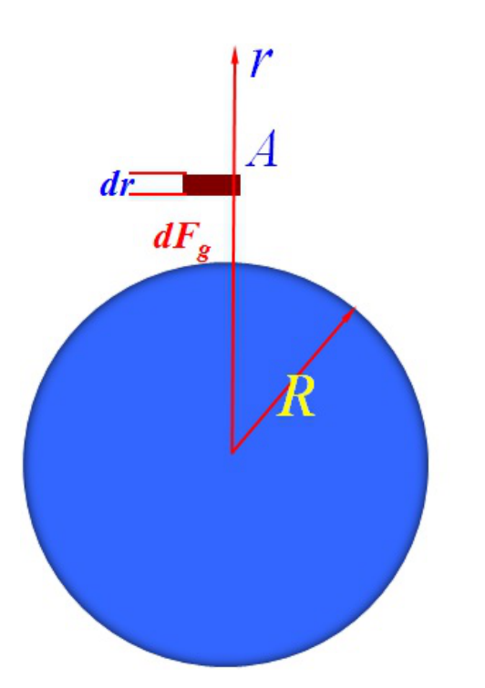
Based on the balance between the gravitational force and the force from the difference of the atmospheric pressure, we obtain
or
(0.5point)
For the ideal gas, we have
Since the atmospheric temperature is constant, Equation (12) can written to be
(0.5point)
Inserting Equation (13) into (11), we have
By integrating Equation (14), we obtain
(0.5point)
Thus, the ration of the atmospheric density at the altitudes H=160km and H=220km is
(0.5point)
(ii)At the altitude H=160km, the collision frequency of atmospheric molecules is
(0.5point)
Since the lifetime of the oxygen atom in the first excited state lasts about 110s, the oxygen atom will collide with other molecules over one hundred times. Thus, the high-frequent collision between particles can de-excite oxygen atoms before they have a chance to radiate. But, the oxygen atoms in the second excited state will emit photons since their lifetime is so short. Thus, aurora at H=160km is resulted from emission of the oxygen atoms in the second excited state. The wavelength is
(0.8point)
The color for this wavelength is green. (0.2point)
At the altitude H=220km, the collision frequency of atmospheric molecules is
(0.5point)
All oxygen atoms in the first and second excited states have a chance to radiate since the collision frequency is so low. Because the number of the oxygen atoms in the first excited state is much larger than in the second excited state, we observe the aurora color is from the emission of the oxygen atoms in the first excited state. The wavelength is
(0.8point)
The color for this wavelength is red. (0.2point)
(g)
Solution for (g)
At the geosynchronous orbit, we have
or
Using , we have
(0.5point)
Using , we have
or
(1.0point)
where is the mass density. At the position , the Earth's dipole magnetic field strength is
From Equation (19), we obtain
(0.5point)
With this speed of the solar wind, the position of the dayside magnetopause is 6.6R at the geosynchronous orbit. Thus, a geosynchronous satellite could be damaged by the solar wind.