Съдържание
УсловиеPart A: Alignment of the setup (0,6 т.)Part B: Diffraction patterns from Sample 2 (0,8 т.)Part C: Diffraction patterns from Sample 3 (0,8 т.)Part D: Theory behind the reflected diffraction patterns from Sample 3 (3,5 т.)Part E: Determination of the unknown angle for Sample 4 (2,2 т.)Part F: Diffraction patterns from Sample 5 (2,4 т.)Part G: Determination of the lattice-plane spacing for ZnSe (1,7 т.)ОтговориРешениеAPhO 2016, Експеримент — Задача 1. Reflected optical diffraction patterns from one-dimensional structures
Asian Physics Olympiad 2016 — Experiment Problem – E1 · 12 т.
Условие
Introduction
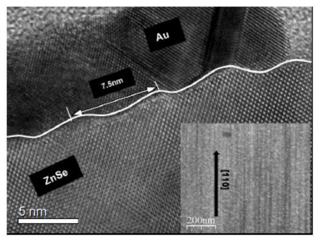
This experiment is based on a recent discovery of a reflected high-energy electron diffraction phenomenon of a nanostructured Zinc-Selenide (ZnSe) surface that not only has a one-dimensional (1D) non-uniform modulation in nanoscale, but also has periodic atomic lattice spacing along the orientation of the 1D nanostructure (Nanotechnology, 20 (21), 215607(2009)). Figure 1 shows the cross-sectional image of the nanostructured ZnSe surface capped with a Au layer while the inset is an image of its surface without the Au cap.
Objective
In this experiment, you are going to explore the optical analogy of this phenomenon for samples with 1D structure on a micrometer scale.
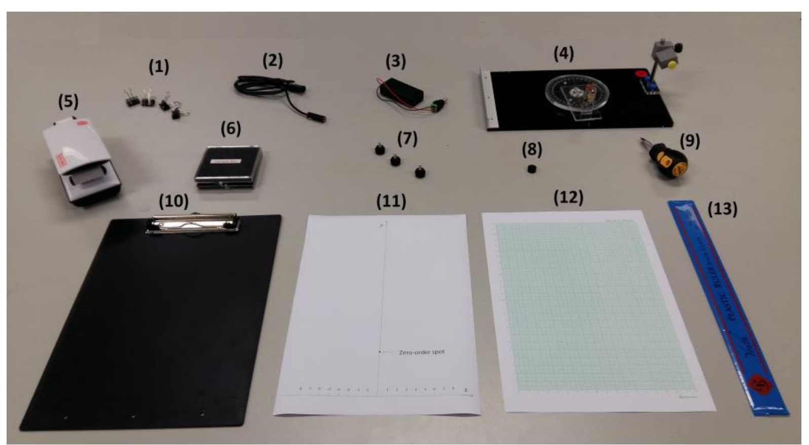
List of apparatus and tools
| [1] | 4 Paper clips |
|---|---|
| [2] | Laser diode |
| [3] | Battery pack with on/off switch |
| [4] | Optical platform with rotary disk, angular scale and laser-diode holder |
| [5] | LED lamp |
| [6] | Sample box containing Samples 1 to 5 |
| [7] | 3 screws for the observation board |
| [8] | Pinhole |
| [9] | Flat-head screw driver |
| [10] | Observation board |
| [11] | Alignment sheet |
| [12] | Graph papers |
| [13] | 30 cm ruler |
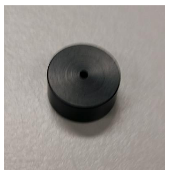
Pictures of key apparatus and tools
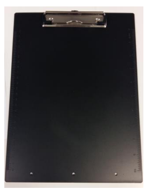
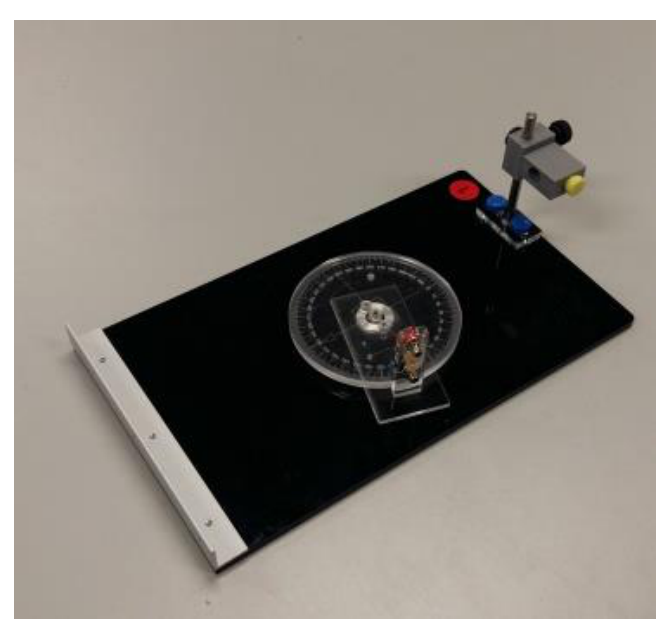
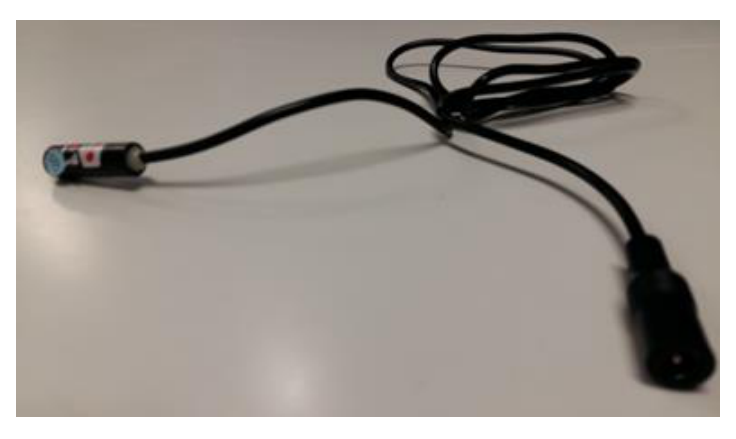
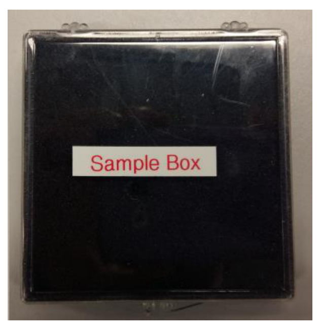
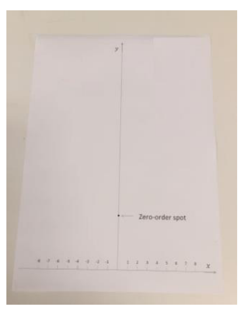
Additional notes for items in the sample box
- All samples used in this experiment are squarely-shaped with dimensions of 1.5 cm × 1.5 cm. They are all labelled from 1 to 5 at one side of each sample holder.
- All sample holders have dimensions of 2.0 cm × 2.0 cm with a reference point marked as a triangle engraved near the center of one edge.
- Before placing each sample on the center of the rotary disk, you should ensure the tip of the arrow on the rotary disk is pointing to the mark of the angular scale. When placing a new sample, try to align it with the square marking on the rotary disk of the platform. The sample position at (only refers to Samples 2 to 5) is defined when the reference point is aligned with and facing the mark on the angular scale.
| Sample | Description of the samples |
|---|---|
| 1 | A plane mirror. |
| 2 | A steel plate having straight scratch grooves parallel to two edges with non-uniform spacing. |
| 3 | A regular grating with the spacing between adjacent grooves equal to , the grating constant. |
| 4 | Similar to Sample 2, but with non-uniformly spaced scratch grooves oriented at an angle of with respect to the line joining the and marks on the angular scale of the rotary disk. |
| 5 | A steel plate that not only has straight scratch grooves with non-uniform spacing, but also has pre-made grooves with equal adjacent spacing . These pre-made grooves lie perpendicularly to the straight scratch grooves with non-uniform spacing. |
Safety precautions and general advice
- Caution: Do not stare into the laser beam directly!!
- Switch off the laser diode when it is not in use to avoid unnecessary draining of the battery.
- Always keep the samples in an upright position. Avoid any contact with the surface of the samples.
- Always hold the edges of the sample holder with your hands, when transferring the samples.
Initial adjustments / procedures
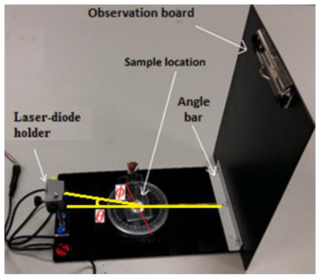
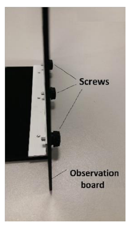
- Construct the experimental setup as shown in Figure 9. The observation board can be attached to the rotary disk using the three screws, as shown in Figure 10.
- Mount the laser diode on the laser-diode holder. [Note: Do not over-tighten the yellow screw when securing the laser diode to the holder; otherwise the laser diode may get damaged.]
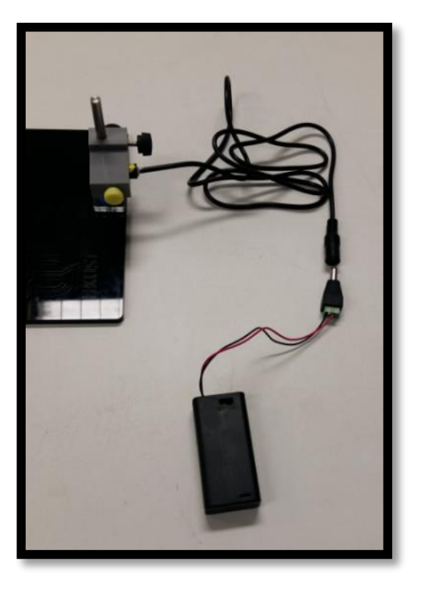
- Connect the battery pack to the laser diode as shown in Figure 11.
- Attach a piece of paper to the observation board to observe the light emitted by the laser diode, then adjust the aperture of the laser diode using a flat-head screw driver to obtain a beam spot of about 1 mm in diameter.
- Place the laser diode in the laser-diode holder such that its head is about 5 to 10 mm out of the holder.
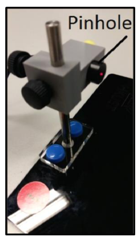
- Attach the provided pinhole to the laser diode as shown in Figure 12, so that the size of the beam spot can be further reduced.
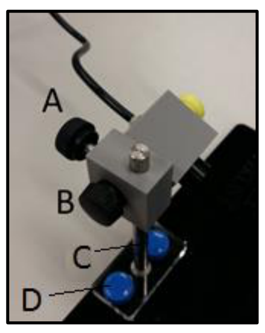
- This experiment requires that the horizontal projection of the laser beam must be aligned with the and marks on the angular scale and the laser beam must hit on the center of the sample being studied. These can be achieved by adjusting the location and tilting angle of the laser-diode holder with the screws as shown in Figure 13.
Experiment
Part A: Alignment of the setup (0,6 т.)
Construct the experimental setup based on Figure 9. Note that the distance between the observation board and the center of the rotary disk has been fixed at 15 cm. Place Sample 1 at the center of the rotary disk following the procedure as described in the additional notes for items in the sample box (Page 3). Attach the alignment sheet to the observation board with the -axis matching with the top edge of the angle bar holding the observation board (This can be done by folding the portion of the paper below the marked -axis backward). The -axis is defined in this way because the experimental setup is designed in a way that the surfaces of all the samples sitting on the rotary disk are aligned with the top edge of this angle bar. In addition, the origin of the -axis must be aligned with the mark on the angular scale. In this experiment, the incident angle of the laser beam is fixed at a certain value. Adjust the height and tilting angle of the laser diode so that the laser beam hits the center of Sample 1 and the spot of the reflected laser beam overlaps with the “zero-order spot” marked on the alignment sheet.
A1 Measure the height of the “zero-order spot” , from the origin of the -axis.
Determine the incident angle of the laser beam from and . Write down the values of in cm and in degrees to three significant figures in the corresponding table in the answer sheet. [0,6 т.]
Part B: Diffraction patterns from Sample 2 (0,8 т.)
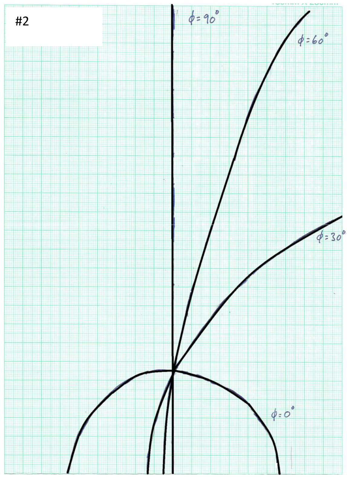
Replace Sample 1 with Sample 2 with the reference point on the sample holder aligned with and facing the mark, in which the direction of non-uniformly spaced scratch grooves of Sample 2 is parallel to the horizontal projection of the laser beam. The angle of rotation of the sample can be adjusted by turning the rotary disk and read from the angular scale.
Attach a graph paper to the observation board. Ensure that the bottom axis of the graph paper matches with the top edge of the angle bar holding the observation board (This can be done by folding the portion of the paper below its bottom axis backward). In addition, the origin of the -axis must be aligned with the mark on the angular scale.
B1 Record the diffraction patterns on the graph paper for , , and of the rotary disk and write down the corresponding angle of rotation next to each pattern. Write down “# 2” at the top of this graph paper. [0,8 т.]
Part C: Diffraction patterns from Sample 3 (0,8 т.)
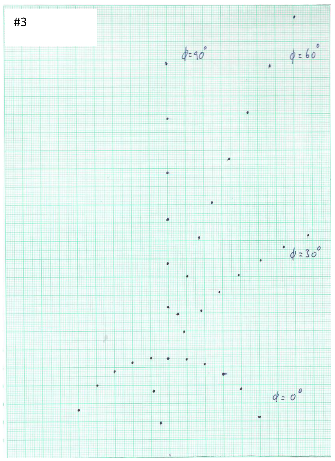
The experiments in this and the next tasks will help you to understand the physics behind the diffraction patterns observed in Task (B1). Remove Sample 2 from the rotary disk and replace it with Sample 3 with the reference point on the sample holder aligned with and facing the mark. For the starting position of Sample 3 (i.e. ), the direction of the grating lines is parallel to the horizontal projection of the laser beam.
Attach a graph paper to the observation board. Ensure that the bottom axis of the graph paper matches with the top edge of the angle bar holding the observation board as described in Part (B). In addition, the origin of the -axis must be aligned with the mark on the angular scale.
C1 Mark the centers of the diffraction spots from Sample 3 for , , and on the graph paper and write down the corresponding angle of rotation next to each pattern. Write down “# 3” at the top of this graph paper. [0,8 т.]
After completing Tasks (B1) and (C1), you should have realized that the reflected diffraction patterns from Sample 2 are continuous while those from Sample 3 are discrete. The reason is that since the spacing between the neighboring straight scratch grooves of Sample 2 is non-uniform, so it is like a grating with its grating constant covers various values. Thus, its diffraction patterns follow the general shapes of the diffraction patterns from a regular grating (like those of Sample 3), however, the diffraction spots become broadened and form the continuous patterns as observed.
Part D: Theory behind the reflected diffraction patterns from Sample 3 (3,5 т.)
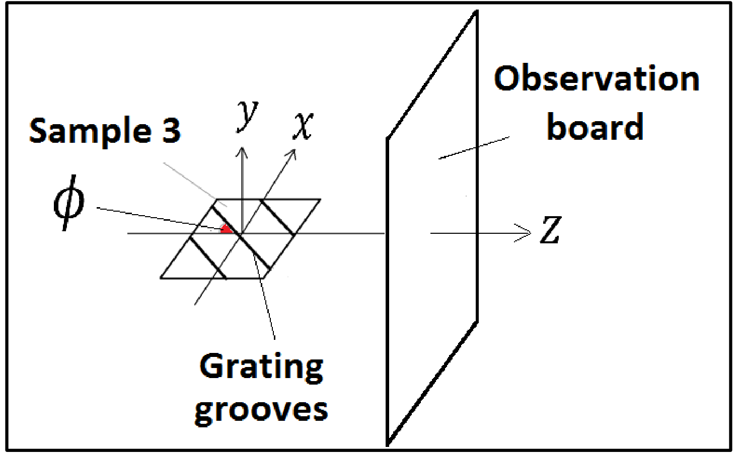
The origin of the reflected diffraction patterns from a regular grating like Sample 3 can be understood with wave optics. In this experiment, we define the -- coordinate system with the origin at the center of the sample as shown in Figure 14.
Using wave optics, one can derive the following equations for the reflected diffraction patterns from Sample 3,
where is the wavelength of the incident laser beam and is the order number of diffraction. One can predict the and co-ordinates of the diffraction spots as a function of using Equations (1) and (2), which can be demonstrated to be consistent with the observed patterns recorded in Task (C1).
Based on Equations (1) and (2), the diffraction spots for should lie along the -axis at with their y-coordinates expressed by the following equation:
D1 Equation (3) can be rearranged to obtain a quadratic equation for the grating constant of Sample 3, as
Derive the expressions for , and . Enter your results in the corresponding table in the answer sheet. [0,9 т.]
D2 By solving this quadratic equation and using the measured values of the diffraction spots for Sample 3 at (See Task (C1)), together with the known values of , and , determine the grating constant of Sample 3 in meters to three significant figures for each diffraction order from the 1st order () up to the 6th order () [Hints: These orders correspond to the six spots above the zero-order spot]. Enter your results in the corresponding table in the answer sheet. [1,8 т.]
D3 Calculate the mean for the grating constant in meters to three significant figures and the standard error of the mean. Enter your results in the corresponding table in the answer sheet. [0,8 т.]
Part E: Determination of the unknown angle for Sample 4 (2,2 т.)
Replace Sample 3 with Sample 4 with the reference point on the sample holder aligned with and facing the mark. In placing Sample 4 onto the rotary disk, the side of its sample holder close to the reference point should be perpendicular to the laser beam.
Attach a graph paper on the observation board. Ensure that the bottom axis of the graph paper matches with the top edge of the angle bar holding the observation board (This can be done by folding the portion of the paper below its bottom axis backward). In addition, the origin of the -axis must be aligned with the mark on the angular scale.
E1 Along the continuous diffracted curve of Sample 4 projected on the graph paper, measure the -coordinates in cm for ten points starting from cm to 3.5 cm with a step of 0.5 cm. Enter your results in the corresponding table in the answer sheet. [0,6 т.]
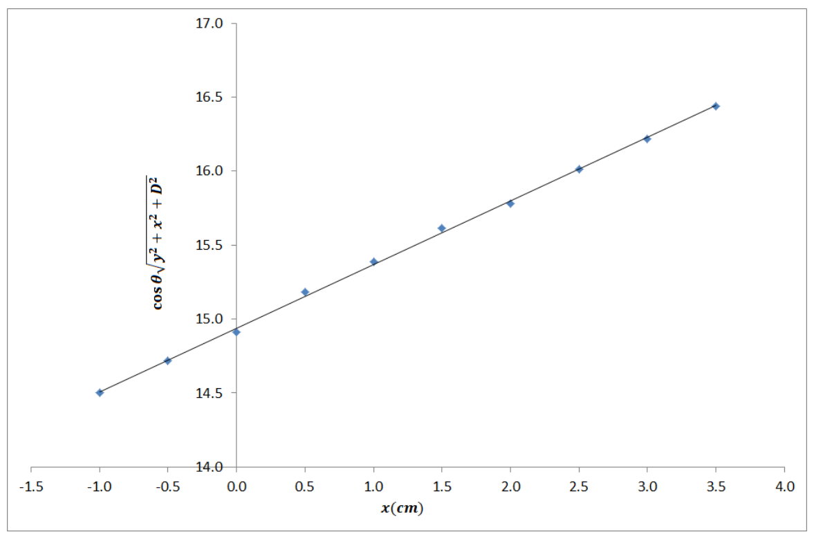
E2 Based on Eq. (1) given in Task (D), construct a linear equation in the form of
Determine the functional forms for , and . Plot against , using the data recorded in E1. Determine the unknown angle in degrees from this graph. Write down all the functional forms and the value of in the corresponding table in the answer sheet. [1,6 т.]
Part F: Diffraction patterns from Sample 5 (2,4 т.)
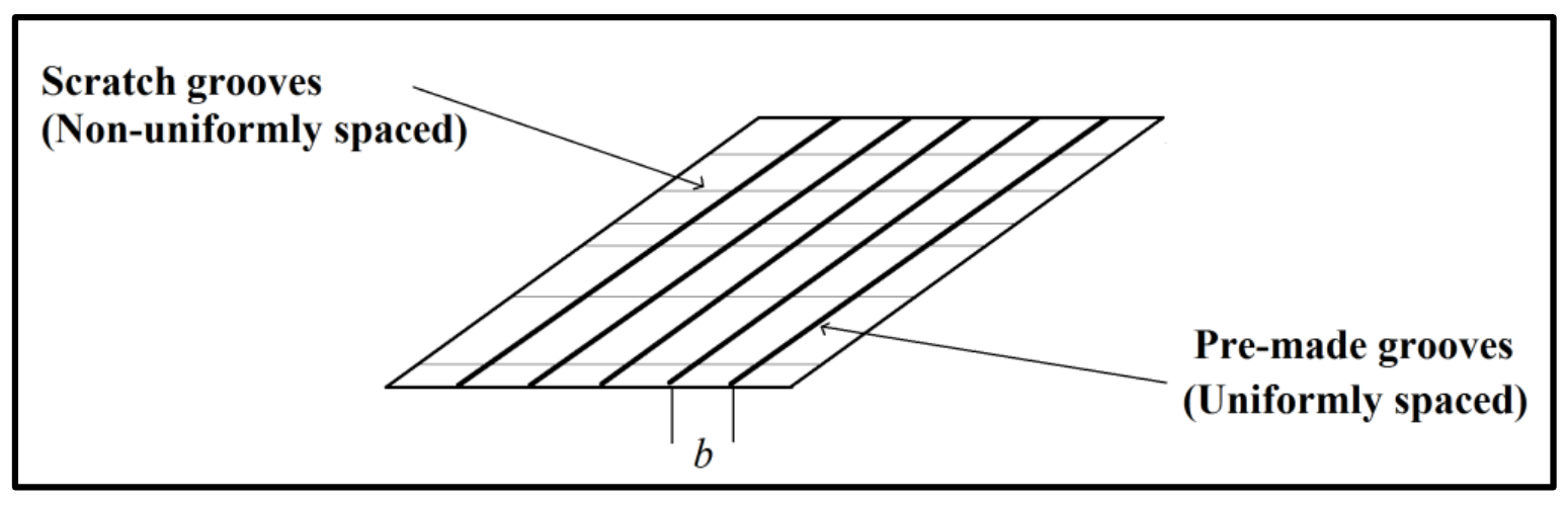
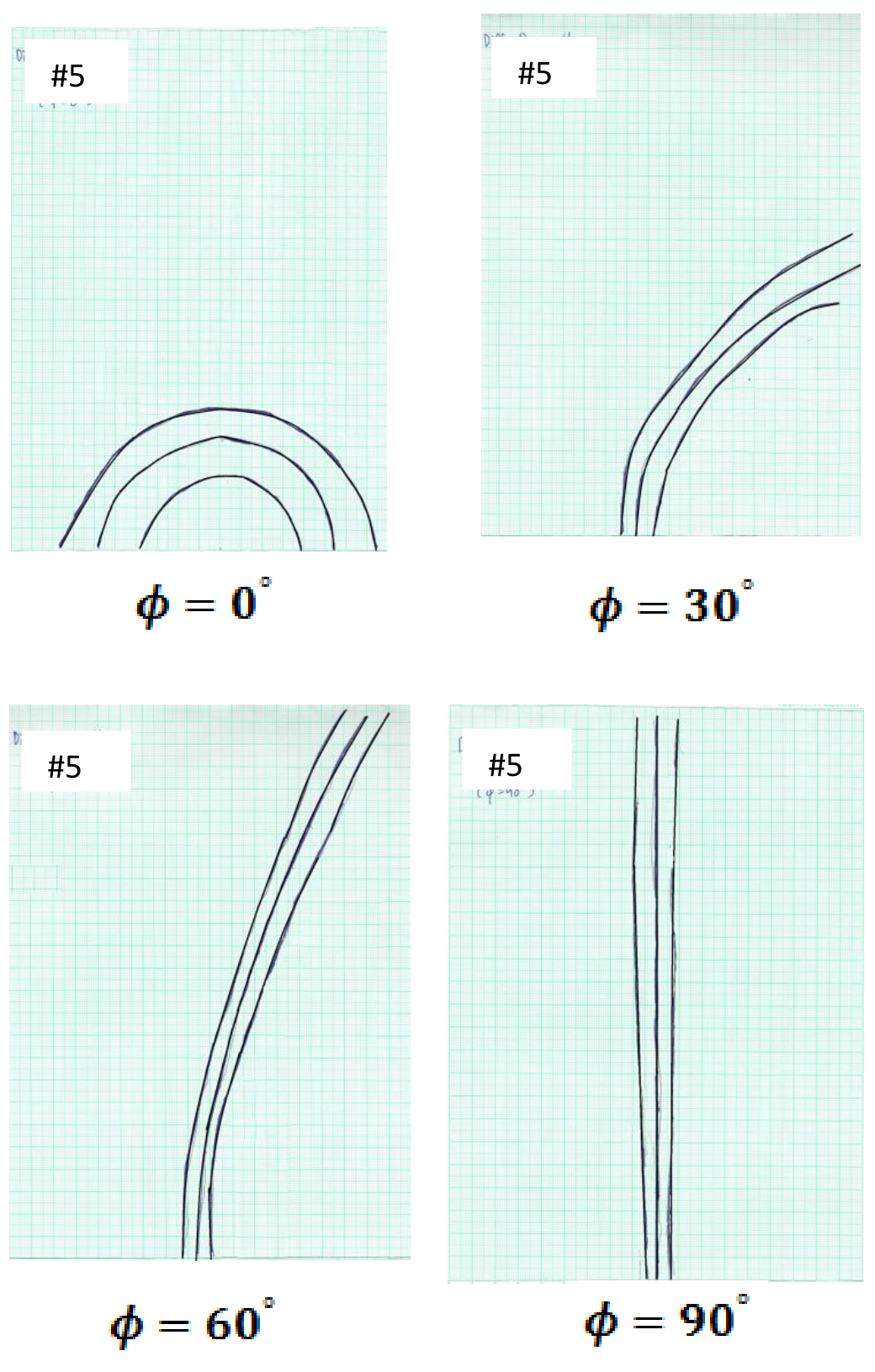
Replace Sample 4 with Sample 5 with the reference point on the sample holder aligned with and facing the mark. The geometry of Sample 5 is shown in Figure 15. For the starting position of Sample 5, the direction of non-uniformly spaced scratch grooves is parallel to the horizontal projection of the laser beam.
Attach a graph paper to the observation board. Ensure that the bottom axis of the graph paper matches with the top edge of the angle bar holding the observation board (This can be done by folding the portion of the paper below its bottom axis backward). In addition, the origin of the -axis must align with the mark on the angular scale.
F1 Record the diffraction patterns you observed for , , and on separate graph papers for each value of . At the top of each graph paper, put down ‘#5’ and the corresponding value. It is expected that you could observe more than 10 diffraction orders. However, you are required to record only three relatively brighter orders on each graph paper. [0,8 т.]
The sample structure of Sample 5 can be considered as a combination of Sample 2 and Sample 3, where the uniformly-spaced pre-made grooves are placed perpendicularly to the scratch grooves with non-uniform spacing. This is an optical analogy of the nano-grating as described in the introduction.
F2 With this understanding, estimate the spacing in meters of the uniformly spaced pre-made grooves of Sample 5 using the recorded diffraction pattern for from Task (F1). Enter the value of in the answer sheet.
[Note that in estimating the value of b, you are only required to take the measured data of the first diffraction order and the estimated b should be rounded up to three significant figures.] [1,6 т.]
Part G: Determination of the lattice-plane spacing for ZnSe (1,7 т.)
As mentioned in the introduction, the above phenomenon was firstly discovered on the reflection high energy electron diffraction (RHEED) patterns of a nanostructured ZnSe surface. Such a surface has a one-dimensional (1D) modulation in nanoscale with non-uniform spatial separation, as well as having periodic atomic lattice planes perpendicular to these nano-grooves. Figure 16 shows the RHEED pattern of such a nanostructured ZnSe surface when the electron-beam is perpendicular to the nano-grooves with non-uniform spacing (Hint: With respect to the periodic atomic lattice planes, such a condition corresponds to )
Note that the spacing of the streaks in this figure, which can be measured using the given scale below the RHEED pattern, matches exactly with the actual diffraction pattern projected on the fluorescence screen (an analogy to the observation board used in this experiment).
In taking the diffraction pattern shown in Figure 16, the accelerating voltage of the electron gun was set to be = 13,000 volts. The corresponding wavelength of the high-energy electrons incident to the center of the sample surface can be calculated by
where the relativistic effect has been taken into account.
The incident angle of the electron beam to the surface of the ZnSe sample is and the distance between the fluorescence screen and the incident spot of the electrons on the nano-structured ZnSe surface is = 26 cm.
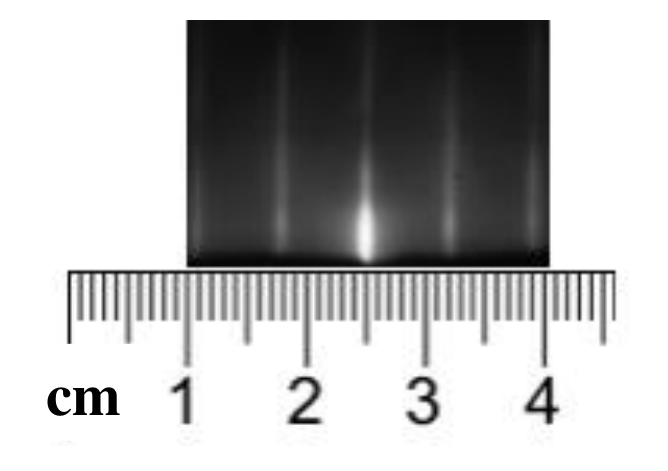
G1 For the ZnSe sample, based on Figure 16 and the experimental conditions given above, determine the lattice-plane spacing of the periodic atomic lattice planes that are perpendicular to the nano-grooves with non-uniform spacing, in meters to three significant figures. Enter your result in the corresponding table in the answer sheet. [1,7 т.]
Отговори
Part A: Alignment of the setup, A1 20.1 °
Official solution: h = 5.50 cm, θ = 20.1°; the marking scheme accepts θ between 19.7° and 20.5°.
Part D: Theory behind the reflected diffraction patterns from Sample 3, D1
Other equivalent forms (e.g. dividing by y² + D²) are accepted by the official marking scheme.
Part D: Theory behind the reflected diffraction patterns from Sample 3, D2 a = 9.95 × 10⁻⁶, 1.03 × 10⁻⁵, 1.04 × 10⁻⁵, 1.04 × 10⁻⁵, 1.03 × 10⁻⁵, 1.05 × 10⁻⁵ m for m = 1 … 6
Only the root a₁ = (−B + √(B² − 4AC))/(2A) is valid; values from the official measurement.
Part D: Theory behind the reflected diffraction patterns from Sample 3, D3 0.0000103 m
Official solution: mean 1.03 × 10⁻⁵ m, standard error of the mean 8 × 10⁻⁸ m.
Part E: Determination of the unknown angle for Sample 4, E2 23.2 °
Official solution: M = cos θ √(y² + x² + D²), I = D, S = tan φ ; slope gives φ = 23.2° (full marks within ±5°).
Part F: Diffraction patterns from Sample 5, F2 0.0000221 m
Official solution with the measured y₁ = 0.0695 m.
Part G: Determination of the lattice-plane spacing for ZnSe, G1 m
Official solution: Δx = 0.7 cm, λ = 0.1067 × 10⁻¹⁰ m, a* = 3.96 × 10⁻¹⁰ m (accepted within ±0.31 × 10⁻¹⁰ m).
Решение
Marking Scheme of E1
(Full Mark = 12 points)
Part A: Alignment of the setup (0,6 т.)
A1
Solution:
The height of the “zero-order spot” is measured to be cm. Using trigonometry,
As cm and cm, one can then fill in the table as follows:
| 5.50 cm | |
|---|---|
Mark
TOTAL = 0.6 points
A1.1 0.2 points for measuring the correct height (between 5.40 cm to 5.60 cm )
A1.2 0.2 points for using the correct equation for determining
A1.3 0.2 points for the correct value of (0.2 points: is between to ) (Otherwise, 0 point)
Part B: Diffraction patterns from Sample 2 (0,8 т.)
B1
Solution:
Mark
TOTAL = 0.8 points
B1.1 0.2 points for the correct sketch of the diffraction pattern for
B1.2 0.2 points for the correct sketch of the diffraction pattern for
B1.3 0.2 points for the correct sketch of the diffraction pattern for
B1.4 0.2 points for the correct sketch of the diffraction pattern for
Part C: Diffraction patterns from Sample 3 (0,8 т.)
C1
Solution:
Mark
TOTAL = 0.8 points
C1.1 0.2 points for the correct sketch of the diffraction pattern for
C1.2 0.2 points for the correct sketch of the diffraction pattern for
C1.3 0.2 points for the correct sketch of the diffraction pattern for
C1.4 0.2 points for the correct sketch of the diffraction pattern for
Part D: Theory behind the reflected diffraction patterns from Sample 3 (3,5 т.)
D1
Solution:
The solution of D1 can be rearranged into the following form
Thus, we have
| C |
Other equivalent forms are also acceptable, such as:
| C |
| C |
Mark
TOTAL = 0.9 points
D1.1 0.3 points for getting the solution of Task (D1) by correct rearrangement
D1.2 0.2 points for the correct form of A
D1.3 0.2 points for the correct form of B
D1.4 0.2 points for the correct form of C
If , and are all correct, then 0.9 points are still given.
D2
Solution:
For each order , we can construct the following table for the coefficients of , and by using the measured value of , the known values of , and (i.e. , and ):
| Order | Measured value of (meters) | |||
|---|---|---|---|---|
| 1 | 0.0835 | |||
| 2 | 0.1075 | |||
| 3 | 0.1315 | |||
| 4 | 0.1580 | |||
| 5 | 0.1875 | |||
| 6 | 0.2180 |
The standard solution for the quadratic equation of is
which leads to two possible solutions, which are
Using the values of , and from the table above, the values of and can be calculated for each order as shown in the following table:
| Order | (meters) | (meters) |
|---|---|---|
| 1 | ||
| 2 | ||
| 3 | ||
| 4 | ||
| 5 | ||
| 6 |
As shown above, all the values of are similar to each other. However, this is not the case for the values of . Thus is not a valid solution for the grating constant and should be discarded.
| Order | Grating constant (meters) |
|---|---|
| 1 | |
| 2 | |
| 3 | |
| 4 | |
| 5 | |
| 6 |
Alternatively, one can also rearrange Equation (3) to the following form:
and then solve for the grating constant accordingly.
Mark
TOTAL = 1.8 points
D2.1 0.4 points for calculating the values of , and for all six orders
D2.2 0.4 points for presenting the correct solution of the quadratic equation
D2.3 0.4 points for providing and for all six orders
D2.4 0.4 points for pointing out that only is the correct solution with explanation
D2.5 0.2 points for the correct values of for all six orders (0.2 points: is within the uncertainty of ±10%) (0.1 points: is within the uncertainty of ±20%) (Otherwise, 0 point)
D3
Solution:
As we have six values of (i.e. ), the mean of the grating constant can be calculated by
For the standard error of the mean for the grating constant, we can use
| Mean of grating constant | |
|---|---|
| Standard error of the mean |
Mark
TOTAL = 0.8 points
D3.1 0.2 points for the correct formula in determining the mean
D3.2 0.2 points for the correct formula in determining the standard error of the mean
D3.3 0.2 points for the correct value of the mean (0.2 points: is within the uncertainty of ±10%, 0.1 points: is within the uncertainty of ±20%, otherwise, 0 point)
D3.4 0.2 points for the correct value of the standard error of the mean (0.2 points: is within the uncertainty of ±10%, 0.1 points: is within the uncertainty of ±20%, otherwise, 0 point)
Part E: Determination of the unknown angle for Sample 4 (2,2 т.)
E1
Mark
TOTAL = 0.6 points
E1 0.6 points for filling in the correct values of -coordinate in the table.
Detailed marking allocation of Task E1 is as follows:
| /cm | /cm ±0.4cm 0.6 pts | /cm ±0.8cm 0.4 pts | /cm ±1.2cm 0.2 pts |
|---|---|---|---|
| -1.0 | 3.1 to 3.9 | 2.7 to 4.3 | 2.3 to 4.7 |
| -0.5 | 4.1 to 4.9 | 3.7 to 5.3 | 3.3 to 5.7 |
| 0.0 | 4.8 to 5.6 | 4.4 to 6.0 | 4.0 to 6.4 |
| 0.5 | 5.6 to 6.4 | 5.2 to 6.8 | 4.8 to 7.2 |
| 1.0 | 6.1 to 6.9 | 5.7 to 7.3 | 5.3 to 7.7 |
| 1.5 | 6.6 to 7.4 | 6.2 to 7.8 | 5.8 to 8.2 |
| 2.0 | 6.9 to 7.7 | 6.5 to 8.1 | 6.1 to 8.5 |
| 2.5 | 7.3 to 8.1 | 6.9 to 8.5 | 6.5 to 8.9 |
| 3.0 | 7.6 to 8.4 | 7.2 to 8.8 | 6.8 to 9.2 |
| 3.5 | 7.9 to 8.7 | 7.5 to 9.1 | 7.1 to 9.5 |
Solution:
| co-ordinate (cm) | co-ordinate (cm) |
|---|---|
| -1.0 | 3.5 |
| -0.5 | 4.5 |
| 0.0 | 5.2 |
| 0.5 | 6.0 |
| 1.0 | 6.5 |
| 1.5 | 7.0 |
| 2.0 | 7.3 |
| 2.5 | 7.7 |
| 3.0 | 8.0 |
| 3.5 | 8.3 |
E2
Solution:
Eq. (1) can be rearranged to get
Take the square root for both sides and then multiply the right hand side by to get
Thus, the above equation can be rewritten as
If one plots versus , the slope of the resulting straight line will be . From the slope, one can find the unknown angle . Using the data from the table below,
| (cm) | (cm) | (cm) | ||
|---|---|---|---|---|
| -1.0 | 3.5 | 15 | 0.939 | 14.494 |
| -0.5 | 4.5 | 15 | 0.939 | 14.713 |
| 0.0 | 5.2 | 15 | 0.939 | 14.907 |
| 0.5 | 6.0 | 15 | 0.939 | 15.177 |
| 1.0 | 6.5 | 15 | 0.939 | 15.379 |
| 1.5 | 7.0 | 15 | 0.939 | 15.607 |
| 2.0 | 7.3 | 15 | 0.939 | 15.777 |
| 2.5 | 7.7 | 15 | 0.939 | 16.005 |
| 3.0 | 8.0 | 15 | 0.939 | 16.210 |
| 3.5 | 8.3 | 15 | 0.939 | 16.430 |
We can then make a plot of vs as shown below:
From the plot, we can estimate the slope to get . (Remark: one can also find out the y-intercept to be cm, which is in good agreement with the value assigned in this experiment.)
Therefore,
Mark
TOTAL = 1.6 points
E2.1 0.3 points for the correct form of
E2.2 0.3 points for the correct form of
E2.3 0.3 points for the correct form of
E2.4 0.4 points for plotting the linear relationship between and
E2.5 0.3 points for the correct value of (0.3 points within the uncertainty of , 0.2 points within the uncertainty of , otherwise, 0 point)
Part F: Diffraction patterns from Sample 5 (2,4 т.)
F1
Mark
TOTAL = 0.8 points
F1.1 0.2 points for the correct sketch of the diffraction pattern for
F1.2 0.2 points for the correct sketch of the diffraction pattern
F1.3 0.2 points for the correct sketch of
F1.4 0.2 points for the correct sketch of
Solution:
F2
Solution:
The formation of the observed diffraction pattern from Sample 5 at can be considered in the following way: the periodic pre-made grooves (perpendicular to the -direction) form a set of discrete diffraction spots lying along the -axis. However, each of these spots is extended to form an arc due to the background straight scratched grooves with non-uniform spacing and thus forming a multi-arc pattern as observed. With this understanding, one can take the peak of the brightest arc as the zero-order (which should be located at cm), and then measure the value of the peak of the 1st order diffraction pattern. This should satisfy Equation (3) as below:
where is the spacing of the pre-made grooves. From the recorded diffraction at for Sample 5, the value of is measured to be 0.0695 m. Similar to what has been done in Task (D1), one can rearrange the equation for to form a quadratic equation as
Where
Again, we take the only valid solution of (See the solution of Task (D3) for detailed explanations) as
Alternatively, one can also rearrange Equation (3) to the following form:
and then solve for the spacing accordingly.
Mark
TOTAL = 1.6 points
F2.1 0.3 points for providing the correct value of (0.3 points: is within the uncertainty of , (0.2 points: is within the uncertainty of Otherwise: 0 marks)
F2.2 0.3 points for quoting Equation (3)
F2.3 0.2 points for quoting the expressions of derived in Task (D2)
F2.4 0.2 points for quoting the expressions of derived in Task (D2)
F2.5 0.2 points for quoting the expressions of derived in Task (D2)
F2.6 0.4 points for providing the correct value of (0.4 points: is within the uncertainty of , 0.2 points: is within the uncertainty of , otherwise, 0 point)
Part G: Determination of the plane spacing for ZnSe (1,7 т.)
G1
Solution:
Recalling Eq. (2) given in Task (D),
For the periodic atomic lattice planes, one has and and so Eq. (2) becomes
where is the lattice plane spacing of the periodic atomic lattice planes that are perpendicular to nano-grooves with non-uniform spacing. Thus the average spacing of the RHEED streaks can be written as
which can be measured from the given RHEED pattern to be 0.7 cm. Given that and can be calculated to be m using Equation (6). Thus, the required lattice plane spacing of ZnSe can be calculated as
Remark: For ZnSe, the actual plane spacing for the corresponding lattice plane is .
Alternatively, you can also consider the corresponding lattice planes of ZnSe as a regular grating, and then using the standard formula for diffraction gratings to obtain the same value of .
Mark
TOTAL = 1.7 points
G1.1 0.4 points for quoting Eq. (2) in Task (D)
G1.2 0.5 points for providing the expression for (from )
G1.3 0.2 points for measuring the correct value of (i.e. 0.7 cm) from the diffraction streaks as shown in Figure 10.
G1.4 0.3 points for the correct value of (i.e. m)
G1.5 0.3 points for the correct value of (0.3 points: is within the uncertainty of m, otherwise, 0 point)
Note: The main source of error in determining is the uncertainty in measuring the spacing of the streaks using a ruler (i.e. m).
Оригинал в Архива: exp1.pdf · официални решения: exp1_sol.pdf