Съдържание

Условие Part A. Alignment of light path (2,4 т.)Part B. Deformation of cantilever beam and deduction of Young’s modulus (2,4 т.)Part C. Double layer cantilever beam (2,6 т.)Part D. Test of molecular-absorption-induced bending of a cantilever beam (2,6 т.)Отговори Решение

APhO 2021, Експеримент — Задача 1. Elasticity of cantilever

Оригинал на условието (PDF)Съобщи за грешка

Всички материали от APhO 2021

Elasticity of cantilever (10 points) · 10 т.

Условие

Please read the general instructions in the separate envelope before you start this problem.

I. Introduction

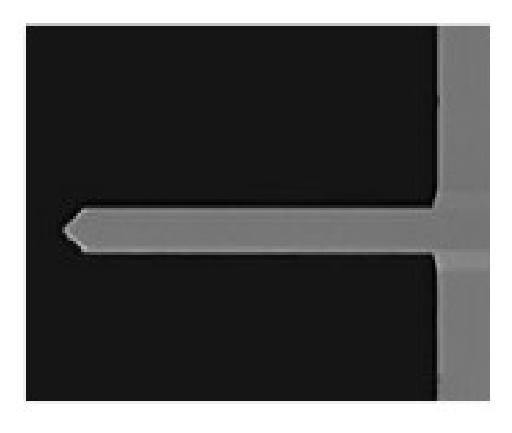
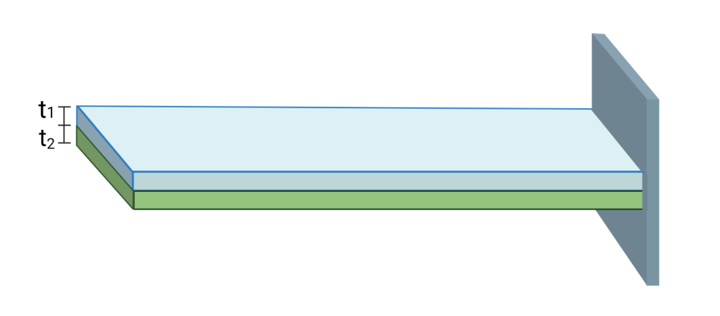
Cantilever beam is one of the common mechanical structures (see Figure 1). It is not only exploited as the main structure to resist shear bending in structure design, but also often seen in the field of nano-engineering. To analyze the elasticity response of nanocantilever beam as well as to elucidate the relationship between stress and strain is important in applied physics. However, it is rather difficult to perform direct measurement of nanomaterials to their mechanical properties. It can be only obtained from the indentation test unlike the uniaxial tensile text in macroscale. For nanocantilever beam subjected to a force by employing an atomic force microscope or nanoindentation, the observation of the flexural deformation of the nanocantilever beam to infer its Young's modulus becomes one of the most important tools for measuring the mechanical properties of materials in microscale.

Figure 1(A): grayscale scanning electron microscope image of a thin horizontal nanocantilever beam with a pointed free end on the left, attached on the right to a vertical support, on a black background. — Figure 1(A) SEM image of a nanocantilever beam

Figure 1(B): 3D sketch of a thin rectangular cantilever plate clamped at its right end to a vertical wall; dimension markers show the length L along the top, the width w along the left edge and the thickness t at the front left corner. — Figure 1(B) illustration of nanocantilever beam, with the length $L$ , width $w$ and thickness $t$ .

II. Introduction of the equipment

Screenshot of simulation program 1A with labelled controls: A Back button, B On/Off switch, C laser emitter, D reflector with position readout E (-20 mm, 20 mm), 22.3°, F PSD detector with position readout G (29 mm, 25 mm), 44.2°, N nano-beam carrier, H PSD recording grid from -1 mm to 1 mm, I Record, J Stop and K Reset buttons, L PSD record chart from -1 mm to 1 mm over 0 to 180 s, M record frequency 1 Hz. — 1A

Common

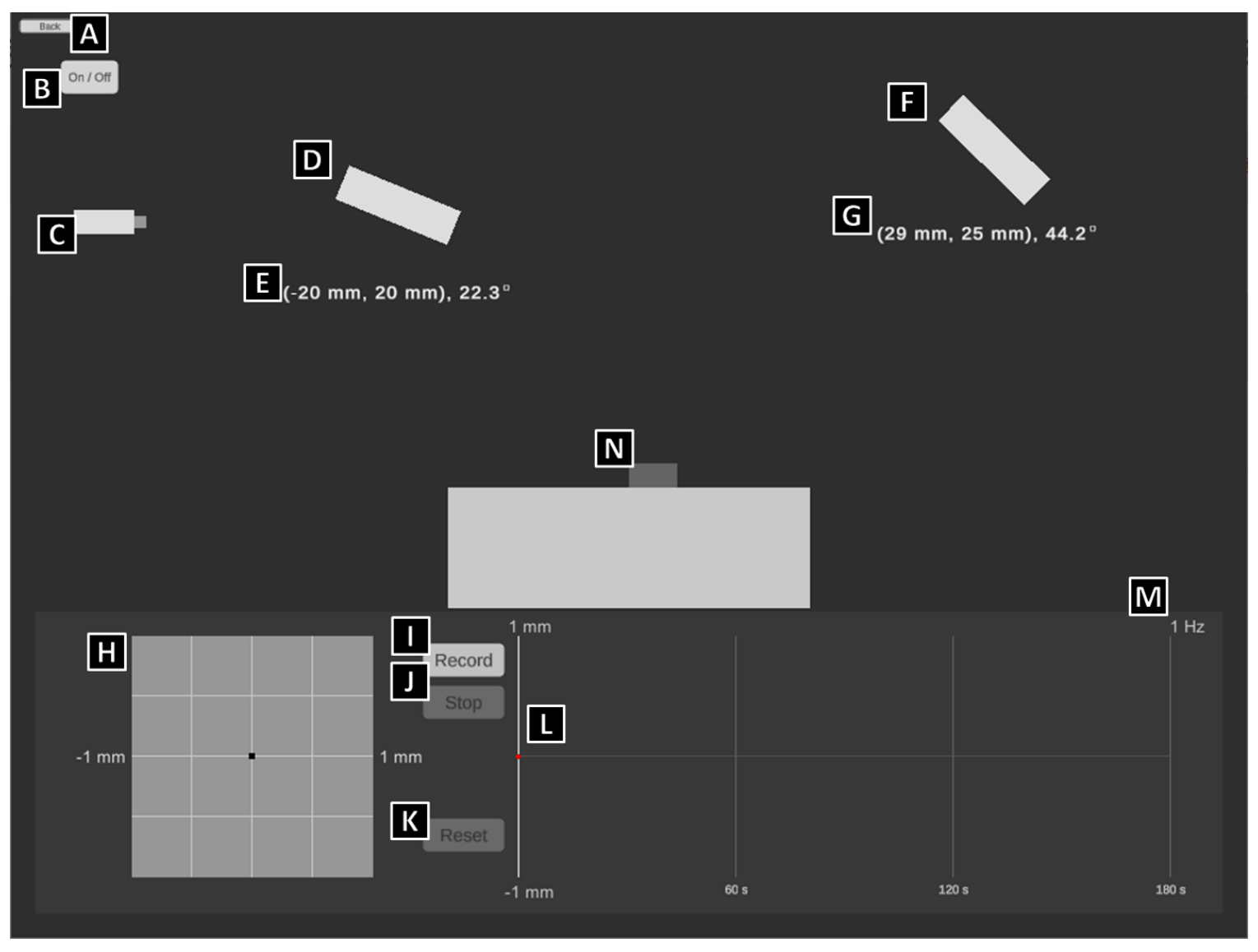
A. Back to previous page
B. Laser switch
C. Laser emitter
D. Reflector: you can control this device precisely by clicking the arrows next to it, or directly dragging it to move with the left mouse button.
E. Position of the reflector: the coordinates are accurate to $1 \times 10^{-3}$ m, and the angle is accurate to 0.1°
F. Position Sensitive Detection, PSD
G. Position of the reflector: the coordinates are accurate to $1 \times 10^{-3}$ m, and the angle is accurate to 0.1°
H. PSD recording system: you can control this device precisely by clicking the arrows next to it, or directly dragging it to move horizontally with the left mouse button. The boundaries of this system are within $\pm 1 \times 10^{-3}$ m both vertically and horizontally.
I. PSD recorder: start-recording button
J. PSD recorder: stop-recording button
K. PSD recorder: reset-recording button
L. PSD record history: the readings are accurate to $0.0001 \times 10^{-3}$ m, which can be recorded with the longest duration of 180 sec. You can query the data with the left mouse button on the chart, or by clicking arrow keys on the keyboard.
M. PSD record frequency: 1 Hz
N. Nano-beam carrier: the coordinates at the left-top corner of the carrier are (0, 0), and the nano-beam would be installed on the left edge of the top.

Screenshot of simulation program 1B: laser, reflector at (-20 mm, 20 mm), 22.3°, PSD at (30 mm, 26 mm), 44.2°, and on the carrier a point-load panel with O the slider from 0 to 10 with a red cursor, P the left/right arrow buttons and Q the force display in nN; the PSD recording grid and chart at the bottom. — 1B

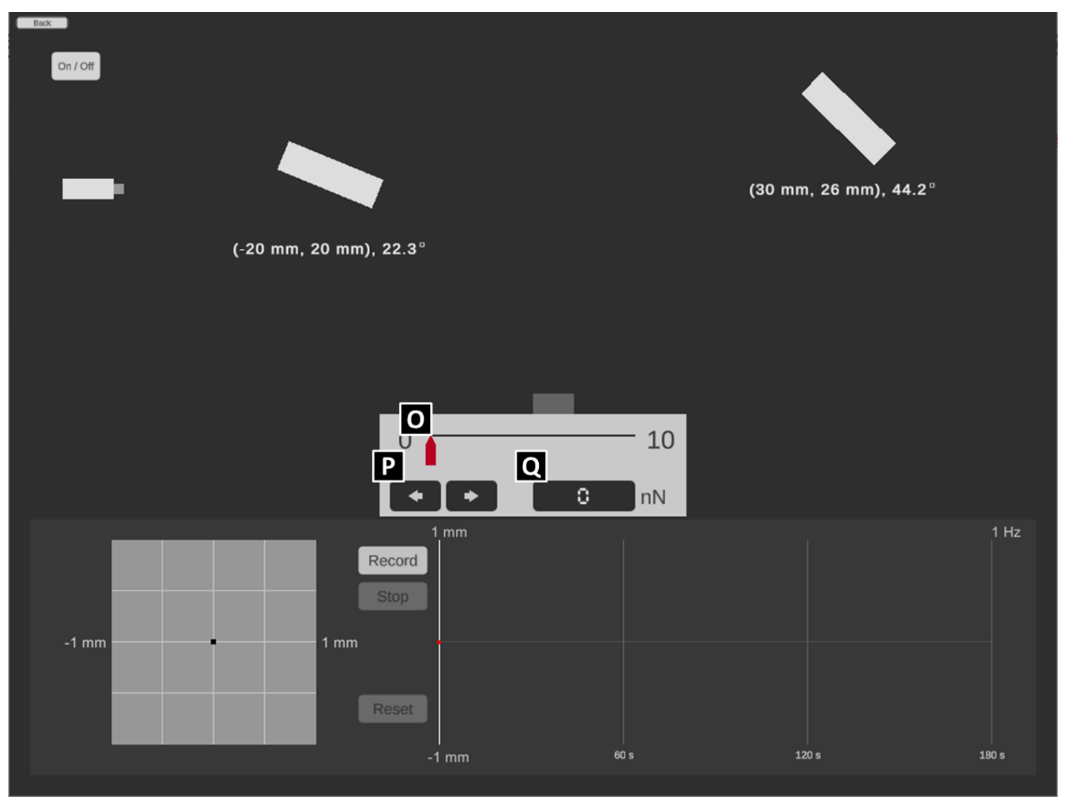
O. the controller of the point load: you can control the force by dragging the red cursor to move horizontally.
P. the micro-controller of the point load: you can control the force precisely by clicking the arrow buttons with the left mouse button.
Q. the monitor of the point load: the precision is up to $0.01 \times 10^{-9}$ N

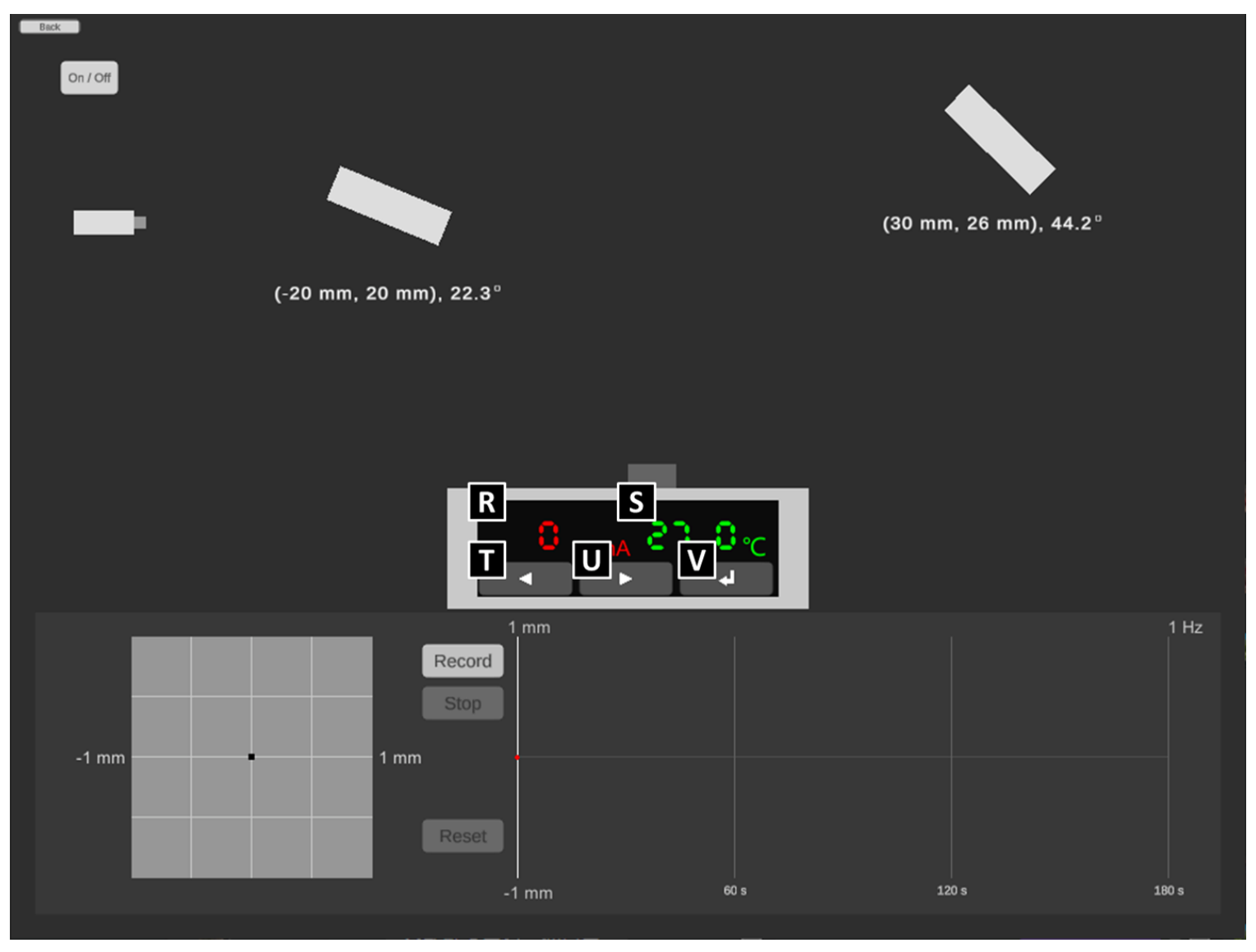
Screenshot of simulation program 1C: laser, reflector at (-20 mm, 20 mm), 22.3°, PSD at (30 mm, 26 mm), 44.2°, and on the carrier a heater panel with R the current display (0 A, red), S the temperature display (27.0 °C, green), T and U the decrease/increase arrow buttons and V the enter button; the PSD recording grid and chart at the bottom. — 1C

R. the monitor of the electric current of the heater with the precision up to $1 \times 10^{-3}$ A.
S. the monitor of the temperature of the heater with the precision up to $0.1^{\circ}$ C
T. the button to decrease current of heater: each click for $2 \times 10^{-3}$ A
U. the button to increase current of heater: each click for $2 \times 10^{-3}$ A
V. the button to set up the change of the electric current: please NOTE that the time to heat or cool down the sample is referring to the authentic experience of the real world and CANNOT be reset arbitrarily, which means the time to let the sample cool down will increase if the sample is over-heated by the excessive electric current.

W. sample switch: switch the test sample by directly clicking it with the left mouse button.

III. Experiment

Note:Please ensure the data and the answers must be expressed by scientific notation and SI unit. The unit of length should be meter.

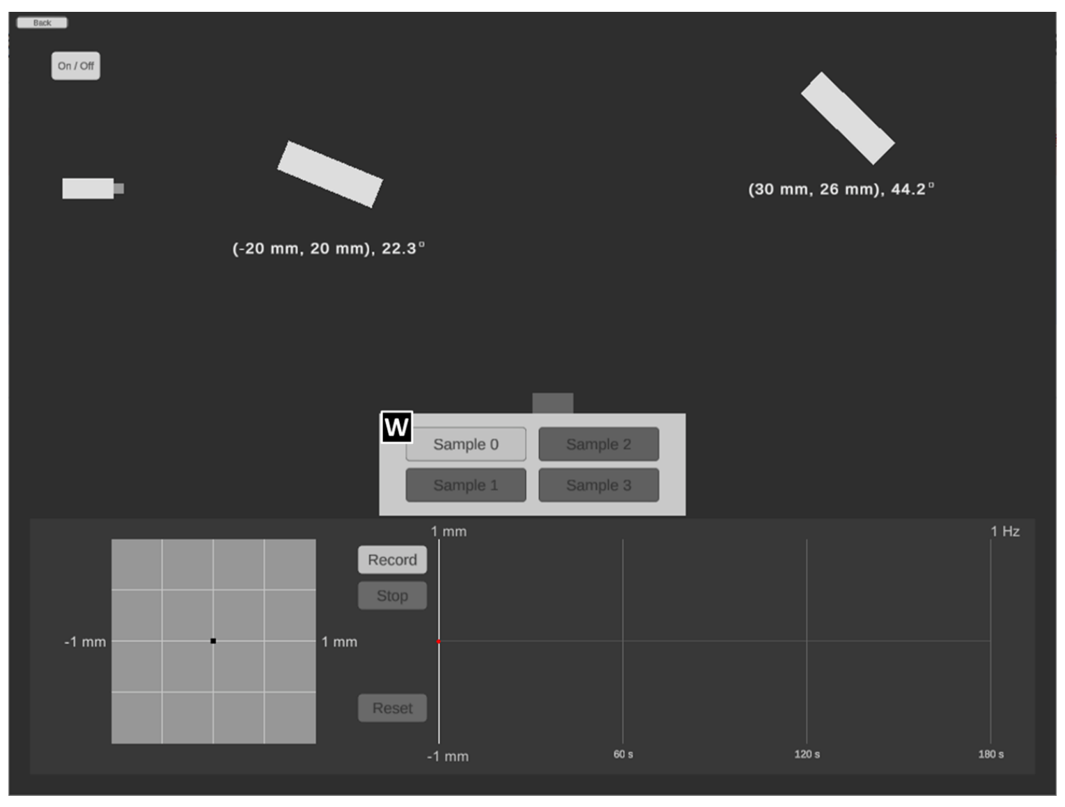
Screenshot of simulation program 1D: laser, reflector at (-20 mm, 20 mm), 22.3°, PSD at (30 mm, 26 mm), 44.2°, and on the carrier W the sample switch with buttons Sample 0, Sample 1, Sample 2 and Sample 3; the PSD recording grid and chart at the bottom. — 1D

Part A. Alignment of light path (2,4 т.)

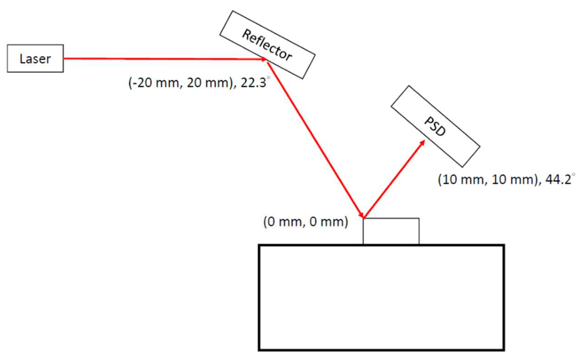
It is not an easy task to measure the deflection of nanocantilever beam at microscopic scale by using optical microscope directly. Therefore, by exploiting the straightness and reflection of laser we are able to measure the reflection by a position sensitive detection sensor (PSD). The length $L$ of the nanocantilever used in the present experiment is about $100 \times 10^{-6}$ m. Please use program 1A and answer question A.1 to A.3.

A.1 Please design a light path so that the laser spot hits the middle of the reflective area of the cantilever beam. Make sure the laser spot can stably appear near the origin of the PSD display screen and draw the relative position (coordinates and angles) of each component on the answer sheet. [0,6 т.]

A.2 Since the cantilever beam will be disturbed when the device turned on, it may take some time to reach a stable state. After the instrument is turned on, the figure of the position of the light spot on the PSD and time will be displayed at the bottom right of the program. Please record the position $d$ of the light spot on the PSD every 3 seconds under external disturbance after pressing the "Record" button. Please record at least 40 data points, and then press the "Stop" button to stop capturing data. [0,8 т.]

A.3 Please use the stable segment of the data obtained by A.2 to find the reference value of measurement of this cantilever beam under the fluctuation of the experimental environment. ( $\bar{d}$ is the average value of $d$ ). [1 т.]

Part B. Deformation of cantilever beam and deduction of Young’s modulus (2,4 т.)

Note : For the convenience of the measurement, we assume the cantilever has reached its stable state under the influence of the environmental perturbation, i.e. the vibration of the optical components will not affect the measured value.

Note:Please ensure the data and the answers must be expressed by scientific notation and SI unit. The unit of length should be meter.

Note:In part B, calculation of the standard deviation in the data analysis is not required.

The Young’s modulus of the material of cantilever beam can be obtained by using an atomic force microscope or a nanoindentation tester to apply an external force to the free end of the cantilever beam. Through the measurement of deformation, the magnitude of Young’s modulus can be obtained. When a force is applied to a nano cantilever beam, if the amount of deformation does not exceed the elastic limit of the material, then the correlation between the force and the deformation of the free end can be formulated as follows:

\delta = \frac{F\,L^3}{3\,E\,I} \qquad (1)

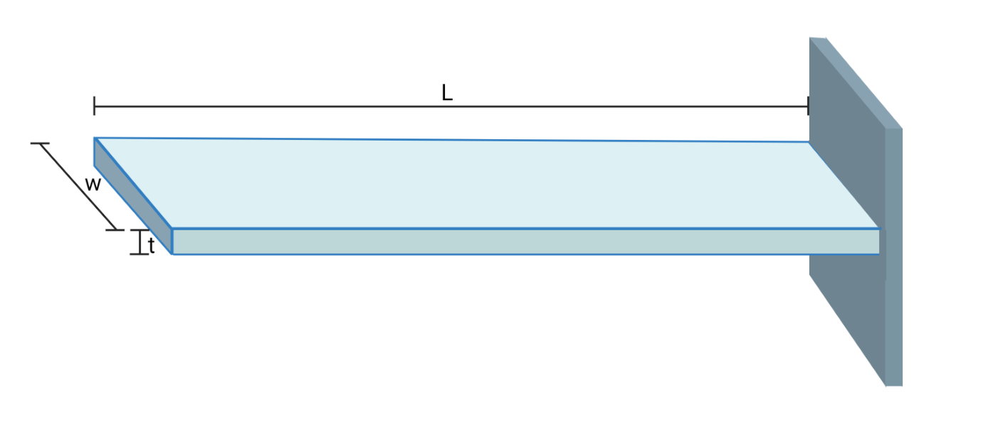
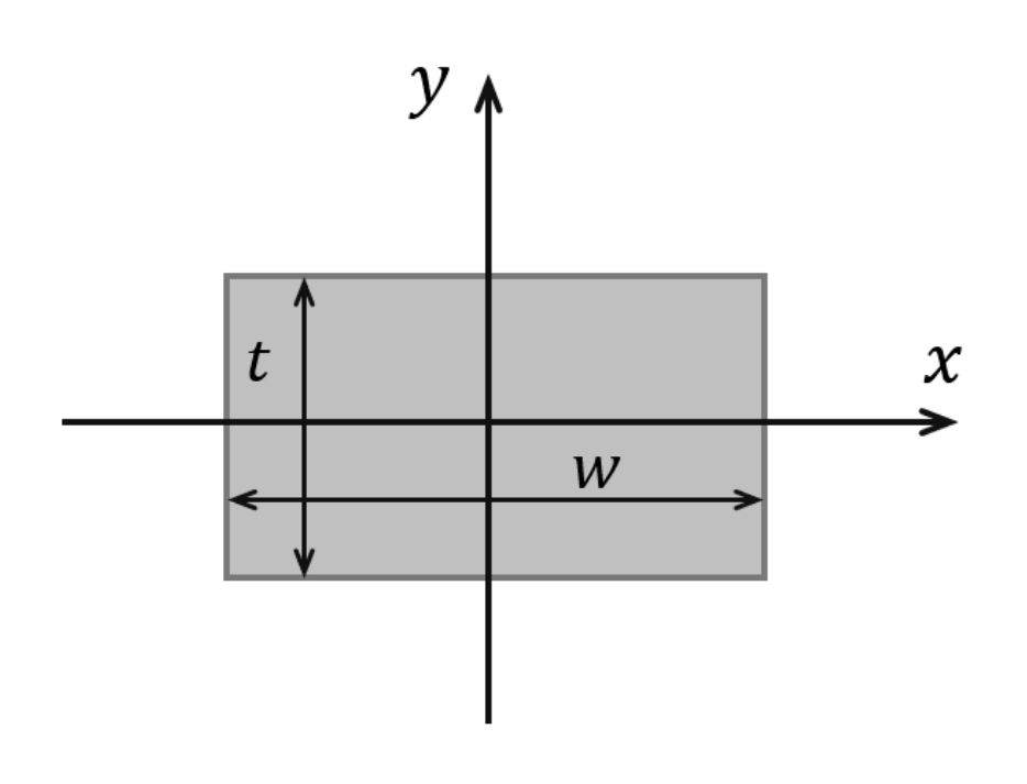
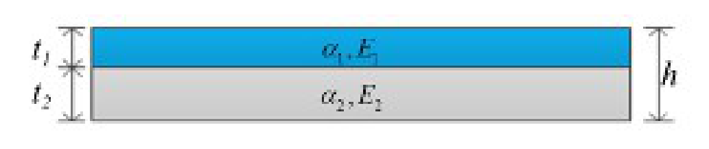
where $F$ is the force applied at the end point, $E$ is the Young’s modulus; $I$ is the area moment of inertia of the cantilever beam section, $L$ is the length of the cantilever beam, and $\delta$ is the magnitude of flexural deformation. The area moment of inertia $I$ is a physical quantity that reflects the influence of the cross-section size on the bending deformation of the cross-section of an object subject to bending deformation. The value of the area moment of inertia can be calculated by simple integration. As shown in Figure 2, there is a cantilever beam whose cross-section height is $t$ , the width is $w$ , and its area moment of inertia can be calculated by integral as follows:

I = \int_A y^2\,dA = \frac{1}{12}w\,t^3 \qquad (2)

The cantilever used in this experiment has an $L$ of $100 \times 10^{-6}$ m, $w$ of $35 \times 10^{-6}$ m, and $t$ of $0.20 \times 10^{-6}$ m. Silicon is used as the substrate material, and its standard Young’s modulus $E$ is $280 \times 10^{9}$ Pa.

Please use program 1B and answer questions B.1 to B.3.

Gray rectangle (beam cross-section) centred on x–y axes, with a vertical double arrow labelled t for the height and a horizontal double arrow labelled w for the width. — Fig. 2 Schematic illustration of the cantilever beam cross-section.

Optical lever: a red laser beam comes from the upper left and reflects off the free end of a micro cantilever (fixed on the right, bent down by δ over length L) towards a tilted Position Sensitive Detector at distance h; a dotted line shows the reflection from the undeformed beam, and the spot shift on the detector is marked d. — Figure 3. Illustration of the optical leverage setup.

B.1 Please design the optical path when the external force is 0 N. Let the laser spot hit in the middle of the reflective area of the cantilever, and be sure about that the laser spot can stably appear near the center of the PSD display screen. Record the data on the table to obtain the measurement reference value $d_0$ . The position of the light spot on the PSD at this time is set as the displacement $\Delta d = 0$ . Then apply five different magnitudes of external forces on the cantilever, and record the experimental results in the table on the answer sheet. [1 т.]

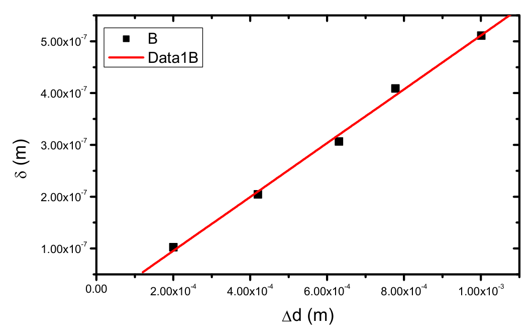
B.2 Fill in the table. Make a plot by taking the magnitude of flexural deformation $\delta$ as the $y$ -axis and $\overline{\Delta d}$ (the average of light spot displacement on the PSD) as the $x$ -axis. [1 т.]

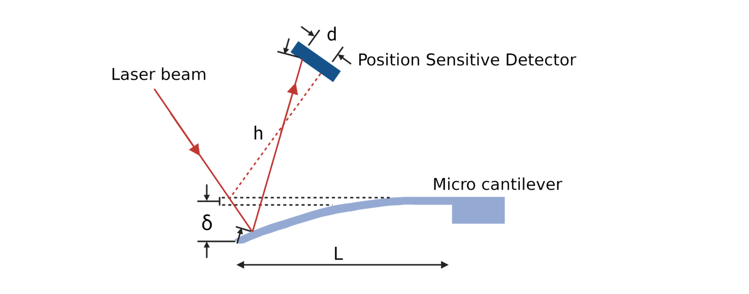
B.3 Please deduce the $C_1$ value value from the optical leverage relationship $\delta = C_1\,\overline{\Delta d}$ , as illustrated in Figure 3. [0,4 т.]

Part C. Double layer cantilever beam (2,6 т.)

Note : For the convenience of the measurement, we assume the cantilever has reached its stable state under the influence of the environmental perturbation., i.e. the vibration of the optical components will not affect the measured value.

Note:Please ensure the data and the answers must be expressed by scientific notation and SI unit. The unit of length should be meter.

Note : In part C, calculation of the standard deviation in the data analysis is not required.

Double layer cantilever beam is a structure often used in nano engineering application (e.g. IC Printed Circuit Board or nano brake). It consists of two layers of different materials which expand at different rate as they are heated. In Timoshenko beam theory, bending stiffness differences were considered. Figure 4 shows a double layer cantilever beam consists of two layers, with thickness $t_1$ and $t_2$ , thermal expansion coefficients $\alpha_1$ and $\alpha_2$ , Young’s modulus $E_1$ and $E_2$ .

According to beam theory, the strain for those two layers could be written as

\gamma_1 = \alpha_1\Delta T + \frac{P_1}{w\,t_1\,E_1} + \frac{t_1}{2\,r} \qquad (3)

\gamma_2 = \alpha_2\Delta T + \frac{P_2}{w\,t_2\,E_2} + \frac{t_2}{2\,r} \qquad (4)

where $P_i$ is the net force, $\Delta T$ is the temperature difference, $w$ is the width, $r$ is the radius of curvature. The net force needs to be balanced as shown in Figure 4. The relation between resultant moment $M$ and net force $P_i$ is written as follows:

M = \sum_i P_i \frac{h}{2} \qquad (5)

The resultant moment $M$ can be written as a function of the bending stiffness $E_iI_i$ and the radius of curvature $r$ , as follows:

M = \sum_i \frac{E_iI_i}{r} \qquad (6)

$E_i$ is Young’s modulus and $I_i$ is moment of inertia. The boundary condition requires the strain to be continuous, that is $\gamma_1 = \gamma_2$ . By this boundary condition, the following equation can be obtained:

\kappa = \frac{1}{r} = \frac{(\alpha_1 - \alpha_2)(T - 300)}{\frac{2}{hw}(\frac{t_1E_1 + t_2E_2}{t_1E_1t_2E_2})(E_1I_1 + E_2I_2) + 0.5h} \qquad (7)

\delta = \kappa\,L^2 \qquad (8)

The double layer beam structure is shown in Figure 5. Parameters for this experiment are listed as follows: $L$ is $100 \times 10^{-6}$ m, $w$ is $35 \times 10^{-6}$ m, $t_2$ is $0.2 \times 10^{-6}$ m, $t_1$ is $0.04 \times 10^{-6}$ m, thermal expansion coefficients $\alpha_1, \alpha_2$ are $14.2 \times 10^{-6}$ /K and $0.8 \times 10^{-6}$ /K; the area moment of inertia $I_1, I_2$ are $1.867 \times 10^{-28}$ m $^4$ and $2.333 \times 10^{-26}$ m $^4$ . The lower layer is silicon base, the Young’s modulus $E$ for silicon is $280 \times 10^{9}$ Pa. Please use program 1C and answer question C.1 to C.3.

Two stacked horizontal layers: a thin blue upper layer labelled α1, E1 with thickness t1 and a thicker gray lower layer labelled α2, E2 with thickness t2; the total thickness is marked h on the right. — Figure 4. schematic illustration of the double layer material used as a cantilever.

3D sketch of a two-layer cantilever plate clamped to a vertical wall on the right: a light blue upper layer of thickness t1 on a green lower layer of thickness t2, with t1 and t2 marked at the free left end. — Figure 5: Double layer beam (Upper layer is metal X. Lower layer is silicon.)

C.1 Please design a simple experiment diagram with light path. Let the laser beam show near the center of the reflected area. Record the data for room temperature, and find the measurement reference $d_0$ , and used this reference as $\Delta d = 0$ . Then, increase the temperature to higher value, wait until the double layer beam stable then record the data. Try to do at least 5 different temperatures and record the data in the table of answer sheet. [1 т.]

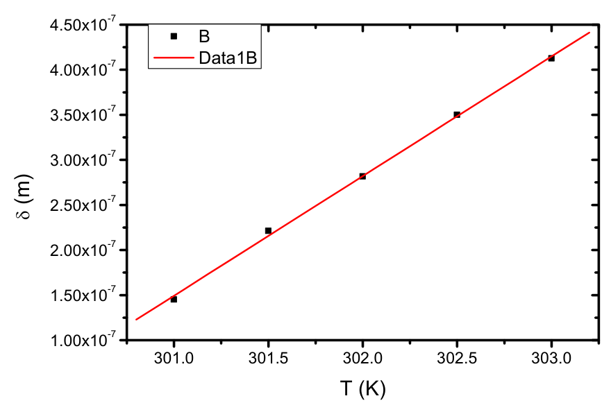
C.2 Fill in the table. Make a plot by taking the magnitude of flexural deformation $\delta$ as the $y$ -axis and the temperature $T$ as the $x$ -axis. By data analysis, find the slope. You can use the correlation between $\delta$ and $\overline{\Delta d}$ in B.3. [1 т.]

C.3 Use data from C.2 to calculate the Young’s modulus for the upper layer material. [0,6 т.]

Part D. Test of molecular-absorption-induced bending of a cantilever beam (2,6 т.)

Note : For the convenience of the measurement, we assume the cantilever has reached its stable state under the influence of the environmental perturbation, i.e. the vibration of the optical components will not affect the measured value.

Note : Please ensure the data and the answers must be expressed by scientific notation and SI unit. The unit of length should be meter.

Note : In part D, calculation of the standard deviation in the data analysis is not required.

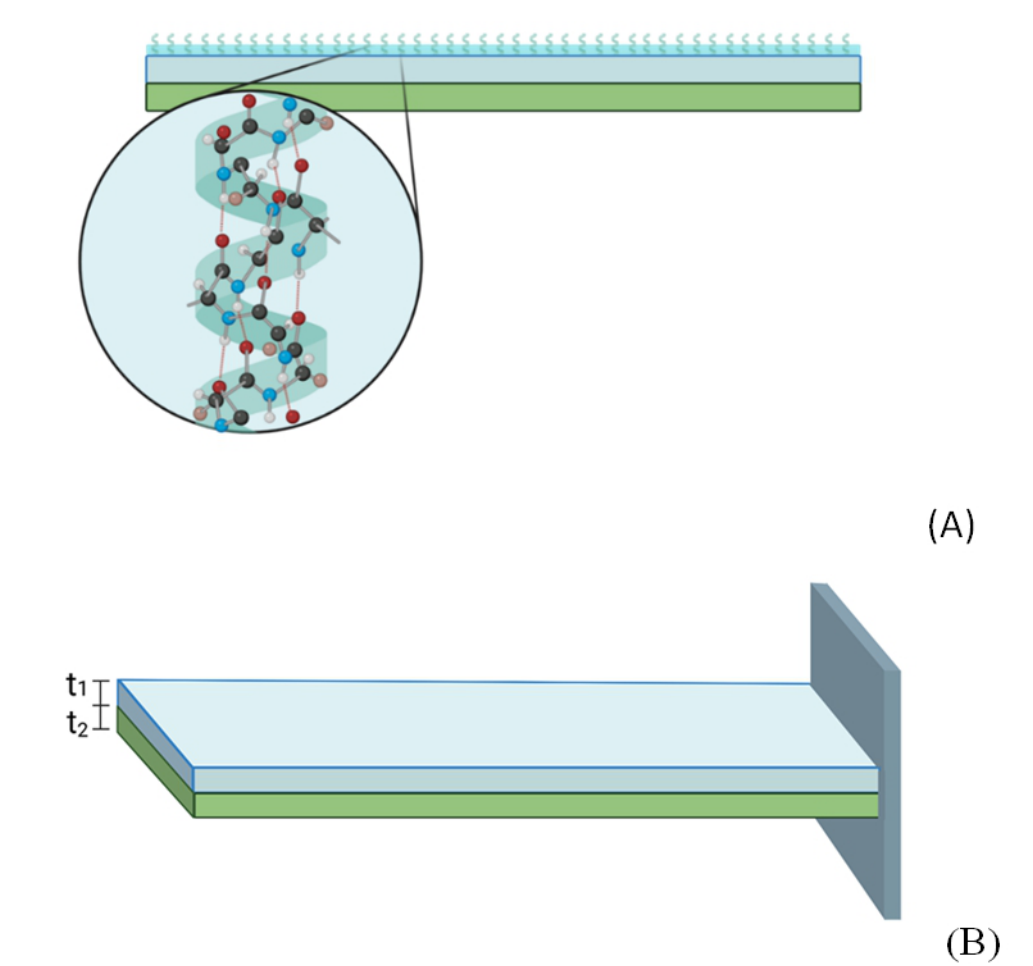
A composited cantilever beam can not only be used as a nano-actuators but also a nano-sensor. As an example, Figure 6 shows a nano-protein sensor consisted of a two-layer cantilever beam on which surface is integrated with microfluidic channels and coated with a protein layer. While a different bio-protein is absorbed onto the cantilever, due to the van-der Waal interactions between the molecules the protein attachment can induce a surface stress which distribution is specific to the uniqueness of protein, and consequently a detectable beam bending.

A schematic diagram of the two-layer cantilever beam used in this experiment is illustrated in Figure 6(B). The length $L$ is about $\sim 100 \times 10^{-6}$ m , $w \sim 35 \times 10^{-6}$ m , $t_2 \sim 0.2 \times 10^{-6}$ m , and $t_1 \sim 0.04 \times 10^{-6}$ m . The lower layer is made by Si as substrate. The Young's modulus of Si is $280 \times 10^{9}$ Pa. The coverage ratio ( $CR$ ) is $\sim 0$ for Sample 0, $\sim 1$ % for Sample 1. You can ignore the effects of the thickness and Young's modulus of the coated molecules on the cantilever beam because of their tiny amount and small $CR$ . Assume the effective bending stiffness $EI^* \approx 1.84 \times 10^{-13}$ N·m $^2$ . Please use program 1D and answer question D.1 to D.4.

(A) A two-layer cantilever strip (light blue upper layer on a green lower layer) with a row of small protein molecules on top, and a circular magnified inset showing a helical protein molecule model. (B) 3D sketch of the two-layer cantilever clamped to a vertical wall on the right, with the layer thicknesses t1 and t2 marked at the free end. — Figure 6. (A) A two-layer cantilever beam, used for nano-sensor. The upper layer is coated with a protein layer. (B) a schematic diagram (not in scale) of the cantilever structure, in which the upper layer is made by metal X and the lower layer by Si.

D.1 Design an optical path for Sample 0, so that the reflected laser spot locates at the center of the reflection zone, i.e. the laser spot appears stable in the origin of the PSD screen. Record the base value $d_0$ measured in the tables of the data sheet. The displacement $\Delta d$ of the laser spot is set zero, $\Delta d = 0$ at this position. Then repeat the experiment with Sample 1. Record your answers on the tables of the data sheet. Note that Sample 1 has the highest coverage ratio ( $CR$ ) in all samples. [0,6 т.]

D.2 Assume the function form of the magnitude of flexural deformation $\delta$ and coverage ratio ( $CR$ ) can be expressed as : $\delta = C_2\frac{CR}{EI^*}L^4$ . Estimate $C_2$ based on your data obtained in D.1. You can use the correlation between $\delta$ and $\overline{\Delta d}$ in B.3. [0,6 т.]

D.3 Use Sample 2 and Sample 3, same molecule but different $CR$ . Measure the spot displacement $\Delta d$ shown on PSD for both samples. Record your answers on the data sheet. [0,8 т.]

D.4 Please estimate $CR$ of Sample 2 and Sample 3 (expressed in %). [0,6 т.]

Отговори

Решение

Part A. Alignment of light path

A1. 0.6 pt

A2. 0.8 pt

time (s)	position $d$ (m)	time (s)	position $d$ (m)	time (s)	position $d$ (m)
3	$-6.415 \times 10^{-4}$	48	$1.198 \times 10^{-4}$	93	$6.85 \times 10^{-5}$
6	$5.261 \times 10^{-4}$	51	$-4.46 \times 10^{-5}$	96	$7.36 \times 10^{-5}$
9	$4.843 \times 10^{-4}$	54	$1.488 \times 10^{-4}$	99	$8.73 \times 10^{-5}$
12	$3.349 \times 10^{-4}$	57	$-7.70 \times 10^{-5}$	102	$7.93 \times 10^{-5}$
15	$-5.386 \times 10^{-4}$	60	$8.75 \times 10^{-5}$	105	$6.39 \times 10^{-5}$
18	$7.91 \times 10^{-5}$	63	$1.604 \times 10^{-4}$	108	$3.22 \times 10^{-5}$
21	$-2.762 \times 10^{-4}$	66	$-1.93 \times 10^{-5}$	111	$6.05 \times 10^{-5}$
24	$1.398 \times 10^{-4}$	69	$1.159 \times 10^{-4}$	114	$3.20 \times 10^{-5}$
27	$-2.039 \times 10^{-4}$	72	$7.10 \times 10^{-5}$	117	$4.71 \times 10^{-5}$
30	$-4.42 \times 10^{-5}$	75	$3.6 \times 10^{-6}$	120	$8.26 \times 10^{-5}$
33	$-1.988 \times 10^{-4}$	78	$-1.79 \times 10^{-5}$
36	$-2.77 \times 10^{-5}$	81	$9.21 \times 10^{-5}$
39	$1.195 \times 10^{-4}$	84	$6.00 \times 10^{-5}$
42	$1.960 \times 10^{-4}$	87	$1.361 \times 10^{-4}$
45	$2.192 \times 10^{-4}$	90	$5.72 \times 10^{-5}$

A3. 1.0 pt

$d$ (m)	$\bar{d}$ (m)	$d - \bar{d}$ (m)	standard deviation
$6.85 \times 10^{-5}$	$6.267 \times 10^{-5}$	$5.5 \times 10^{-6}$	$1.88 \times 10^{-5}$
$7.36 \times 10^{-5}$		$1.09 \times 10^{-5}$
$8.73 \times 10^{-5}$		$2.46 \times 10^{-5}$
$7.93 \times 10^{-5}$		$1.66 \times 10^{-5}$
$6.39 \times 10^{-5}$		$1.2 \times 10^{-6}$
$3.22 \times 10^{-5}$		$-3.05 \times 10^{-5}$
$6.05 \times 10^{-5}$		$-2.2 \times 10^{-6}$
$3.20 \times 10^{-5}$		$-3.07 \times 10^{-5}$
$4.71 \times 10^{-5}$		$-1.56 \times 10^{-5}$
$8.26 \times 10^{-5}$		$1.99 \times 10^{-5}$

reference value of measurement (with standard deviation)：

$6.267 \times 10^{-5} \pm 1.88 \times 10^{-5}$ m

Sample light path for A1: a Laser box on the left sends a horizontal red beam to a tilted Reflector at (-20 mm, 20 mm), 22.3°; the beam reflects down to the beam tip at (0 mm, 0 mm) on top of the carrier block and then up to the tilted PSD at (10 mm, 10 mm), 44.2°. — A1.

Part B. Deformation of cantilever beam and deduction of Young’s modulus

B1. answer sheet. 1.0 pt

$F$ (N)	$d$ (m)	$\bar{d} = d_0$ (m)
0	$-1.82 \times 10^{-5}$	$-1.386 \times 10^{-5}$
	$-1.09 \times 10^{-5}$
	$-6.69 \times 10^{-5}$
	$1.72 \times 10^{-5}$
	$9.5 \times 10^{-6}$

$F$ (N)	$d - d_0 = \Delta d$ (m)	$\overline{\Delta d}$ (m)
$2.00 \times 10^{-9}$	$1.9136 \times 10^{-4}$	$2.0046 \times 10^{-4}$
	$2.0016 \times 10^{-4}$
	$1.9766 \times 10^{-4}$
	$2.0096 \times 10^{-4}$
	$2.1216 \times 10^{-4}$
$4.00 \times 10^{-9}$	$4.2336 \times 10^{-4}$	$4.2018 \times 10^{-4}$
	$4.1536 \times 10^{-4}$
	$4.3526 \times 10^{-4}$
	$4.0346 \times 10^{-4}$
	$4.2346 \times 10^{-4}$
$6.00 \times 10^{-9}$	$6.4136 \times 10^{-4}$	$6.3112 \times 10^{-4}$
	$6.4646 \times 10^{-4}$
	$6.4256 \times 10^{-4}$
	$6.2186 \times 10^{-4}$
	$6.0336 \times 10^{-4}$
$8.00 \times 10^{-9}$	$7.1906 \times 10^{-4}$	$7.7770 \times 10^{-4}$
	$7.8006 \times 10^{-4}$
	$8.0506 \times 10^{-4}$
	$7.7736 \times 10^{-4}$
	$8.0696 \times 10^{-4}$
$1.000 \times 10^{-8}$	$1.01216 \times 10^{-3}$	$1.00106 \times 10^{-3}$
	$1.00076 \times 10^{-3}$
	$1.00336 \times 10^{-3}$
	$9.7846 \times 10^{-4}$
	$1.01076 \times 10^{-3}$

B2. 1.0 pt

$F$ (N)	$\delta$ (m)	$\overline{\Delta d}$ (m)
$2.00 \times 10^{-9}$	$1.022 \times 10^{-7}$	$2.0046 \times 10^{-4}$
$4.00 \times 10^{-9}$	$2.044 \times 10^{-7}$	$4.2018 \times 10^{-4}$
$6.00 \times 10^{-9}$	$3.066 \times 10^{-7}$	$6.3112 \times 10^{-4}$
$8.00 \times 10^{-9}$	$4.088 \times 10^{-7}$	$7.7770 \times 10^{-4}$
$1.000 \times 10^{-8}$	$5.109 \times 10^{-7}$	$1.00106 \times 10^{-3}$

B3. 0.4 pt

$C_1 = 5.196 \times 10^{-4}$

Graph of δ (m) from 0 to 5.00x10^-7 against Δd (m) from 0.00 to 1.00x10^-3: five black square data points (legend B) close to a red fitted straight line (legend Data1B) rising from lower left to upper right. — B2.

Part C. Double layer cantilever beam

C1. 1.0 pt

$T$ (K)	$d$ (m)	$\bar{d} = d_0$ (m)
300	$-2.28 \times 10^{-5}$	$-2.836 \times 10^{-5}$
	$-7.24 \times 10^{-5}$
	$-1.61 \times 10^{-5}$
	$-2.84 \times 10^{-5}$
	$-2.1 \times 10^{-6}$

$T$ (K)	$d - d_0 = \Delta d$ (m)	$\overline{\Delta d}$ (m)
301	$2.8506 \times 10^{-4}$	$2.7928 \times 10^{-4}$
	$2.7186 \times 10^{-4}$
	$2.7466 \times 10^{-4}$
	$2.7436 \times 10^{-4}$
	$2.9046 \times 10^{-4}$
301.5	$4.1276 \times 10^{-4}$	$4.2568 \times 10^{-4}$
	$4.1336 \times 10^{-4}$
	$4.6276 \times 10^{-4}$
	$4.3956 \times 10^{-4}$
	$3.9996 \times 10^{-4}$
302	$5.4146 \times 10^{-4}$	$5.4186 \times 10^{-4}$
	$5.4676 \times 10^{-4}$
	$5.3386 \times 10^{-4}$
	$5.6706 \times 10^{-4}$
	$5.2016 \times 10^{-4}$
302.5	$6.9866 \times 10^{-4}$	$6.7330 \times 10^{-4}$
	$6.6726 \times 10^{-4}$
	$6.6416 \times 10^{-4}$
	$6.8296 \times 10^{-4}$
	$6.5346 \times 10^{-4}$
303	$7.6026 \times 10^{-4}$	$7.9410 \times 10^{-4}$
	$7.7046 \times 10^{-4}$
	$7.9706 \times 10^{-4}$
	$8.1346 \times 10^{-4}$
	$8.2926 \times 10^{-4}$

C2. 1.0 pt

$T$ (K)	$\overline{\Delta d}$ (m)	$\delta$ (m)
301	$2.7928 \times 10^{-4}$	$1.451 \times 10^{-7}$
301.5	$4.2568 \times 10^{-4}$	$2.212 \times 10^{-7}$
302	$5.4186 \times 10^{-4}$	$2.816 \times 10^{-7}$
302.5	$6.7330 \times 10^{-4}$	$3.499 \times 10^{-7}$
303	$7.9410 \times 10^{-4}$	$4.127 \times 10^{-7}$

Slope: $1.337 \times 10^{-7}$

C3. 0.6 pt

$4.98 \times 10^{10}\ \mathrm{N/m^2}\ (Pa)$

Graph of δ (m) from 1.00x10^-7 to 4.50x10^-7 against T (K) from 301.0 to 303.0: five black data points (legend B) on a red fitted straight line (legend Data1B) rising to the right. — C2.

Part D. Test of molecular-absorption-induced bending of a cantilever beam

D1. 0.6 pt

	$d$ (m)	$\bar{d} = d_0$ (m)
Sample 0	$3.4 \times 10^{-6}$	$-7.2 \times 10^{-6}$
	$-1.15 \times 10^{-5}$
	$-1.61 \times 10^{-5}$
	$2.09 \times 10^{-5}$
	$-3.25 \times 10^{-5}$

	$d - d_0 = \Delta d$ (m)	$\overline{\Delta d}$ (m)
Sample 1	$-8.2414 \times 10^{-4}$	$-8.2552 \times 10^{-4}$
	$-8.2884 \times 10^{-4}$
	$-8.2794 \times 10^{-4}$
	$-8.1934 \times 10^{-4}$
	$-8.2584 \times 10^{-4}$

D2. Assume the function form of the displacement and coverage ratio (CR) can be expressed as： $\delta = C_2\frac{CoverageRatio}{EI^*}L^4$ . Estimate $C_2$ based on your data obtained in A9. You can use the correlation between $\delta$ and $\overline{\Delta d}$ in A6. 0.6 pt

$-7.89 \times 10^{-2}$

D3. 0.8 pt

	$d - d_0 = \Delta d$ (m)	$\overline{\Delta d}$ (m)
Sample 2	$-6.1734 \times 10^{-4}$	$-6.0866 \times 10^{-4}$
	$-6.0434 \times 10^{-4}$
	$-6.0054 \times 10^{-4}$
	$-5.9884 \times 10^{-4}$
	$-6.2224 \times 10^{-4}$
Sample 3	$-2.4924 \times 10^{-4}$	$-2.4588 \times 10^{-4}$
	$-2.6224 \times 10^{-4}$
	$-2.4764 \times 10^{-4}$
	$-2.4854 \times 10^{-4}$
	$-2.2174 \times 10^{-4}$

D4. 0.6 pt

Sample 2: 0.738%

Sample 3: 0.298%

Оригинал в Архива: E1 Q English.pdf · официални решения: E1 Solution.pdf