Съдържание

APhO 2021, Теория — Задача 1. Water-Hammer Effect

Оригинал на условието (PDF)Съобщи за грешка

Всички материали от APhO 2021

Theory Q1 — Water-Hammer Effect — Asian Physics Olympiad 2021 TAIPEI — English (Official) · 10 т.

Условие

Introduction

This problem studies variations of fluid pressure caused by pressure waves in a flow pipe. Proposed tasks mainly deal with the water-hammer effect arising from both fast and slow closings of a flow-control valve in the pipe.

We consider only nonviscous liquids and liquid flows which are essentially one-dimensional. All pipes including their valves are assumed to be rigid, but liquids are not always considered to be incompressible. If a liquid element of volume $V_0$ at equilibrium under pressure $P_0$ is subjected to a change of pressure $\Delta P$ , the change of its volume $\Delta V$ is assumed to be proportional to $\Delta P$ so that

\Delta P = -B\,\frac{\Delta V}{V_0} \qquad (1)

The constant of proportionality $B$ represents the bulk modulus of the liquid. For water, take $\rho_0 = 1.0\times 10^3\ \mathrm{kg/m^3}$ as its equilibrium density and $B = 2.2\ \mathrm{GPa}$ .

Part A. Excess Pressure and Propagation of Pressure Wave (2.2 points)

In a uniform cylindrical pipe of length $L$ , water is flowing steadily along the $+x$ direction with horizontal velocity $v_0$ , density $\rho_0$ , and pressure $P_0$ . As shown in Fig. 1, the pipe is connected to a reservoir at a depth $h$ and opens into the atmosphere at pressure $P_\mathrm{a}$ .

Suppose the flow-control valve T at the end of the pipe is then shut instantly so that the oncoming liquid element next to the valve suffers both a pressure change $\Delta P_\mathrm{s} \equiv P_1 - P_0$ and a velocity change $\Delta v = v_1 - v_0$ with $v_1 \le 0$ . This causes a longitudinal wave of excess pressure $\Delta P_\mathrm{s}$ to travel upstream in the $-x$ direction with a speed of propagation $c$ .

Reservoir on the left with free surface at atmospheric pressure P_a and depth h marked by a vertical double arrow; a horizontal pipe from entrance B to end A of length L carries liquid with ρ0, P0 and velocity v0 to the right; valve T at end A opens into the atmosphere at P_a; an arrow x points in the flow direction. — Fig. 1: Steady flow in a uniform pipe.

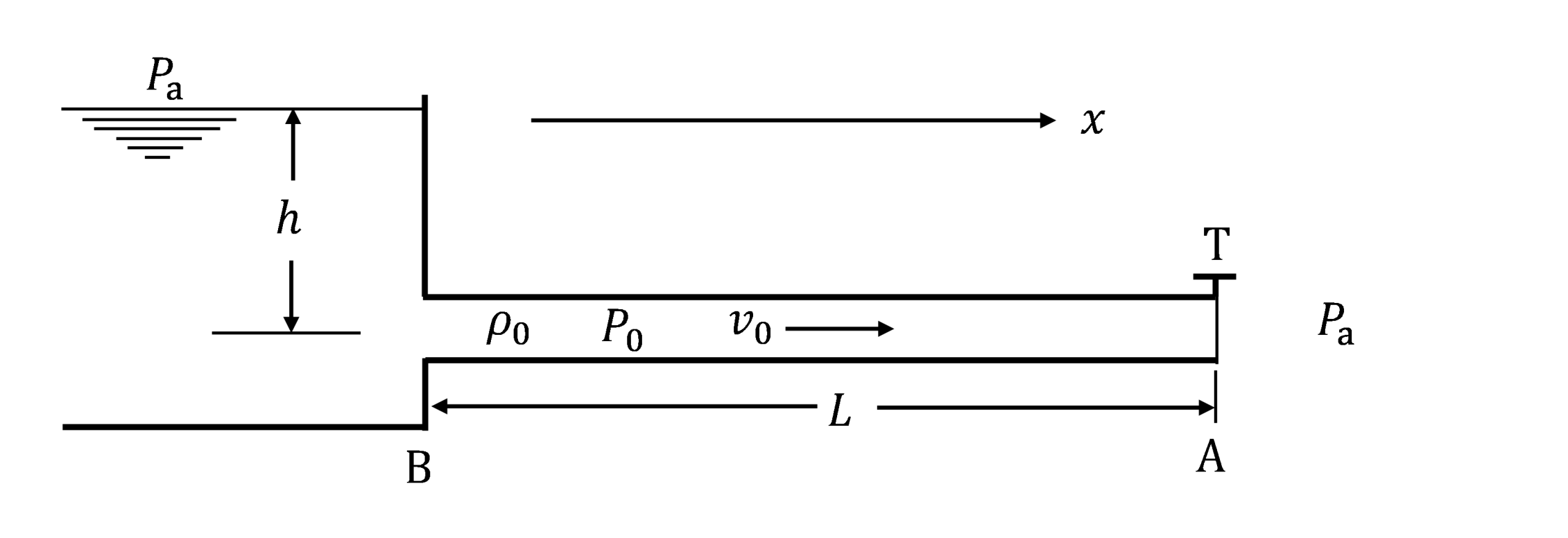
A.1 The excess pressure $\Delta P_\mathrm{s}$ is related to the velocity change $\Delta v$ by $\Delta P_\mathrm{s} = \alpha\rho_0 c\Delta v$ . The speed of propagation $c$ is given by $c = \beta + \sqrt{\gamma B/\rho_0}$ . Find $\alpha$ , $\beta$ , and $\gamma$ . [1,6 т.]

A.2 Calculate values of $c$ and $\Delta P_\mathrm{s}$ for the case of water flow with $v_0 = 4.0\ \mathrm{m/s}$ and $v_1 = 0$ . [0,6 т.]

Part B. A Model for the Flow-control Valve (1.0 points)

Fig. 2 shows a model for control valve T and the liquid flow through it. The valve is taken to be a short section of length $\Delta L$ and inner radius $R$ near the end A of the pipe. Its cone-shaped outlet has an orifice of radius $r$ and opens into the atmosphere at pressure $P_\mathrm{a}$ . Effects of gravity on the efflux are to be neglected.

The liquid is to be regarded as incompressible and the flow as steady with liquid element at the valve inlet having velocity $v_\mathrm{in}$ , pressure $P_\mathrm{in}$ , and density $\rho_0$ . In Fig. 2, stream lines and normal lines are drawn only as an aid for visualizing the flow pattern.

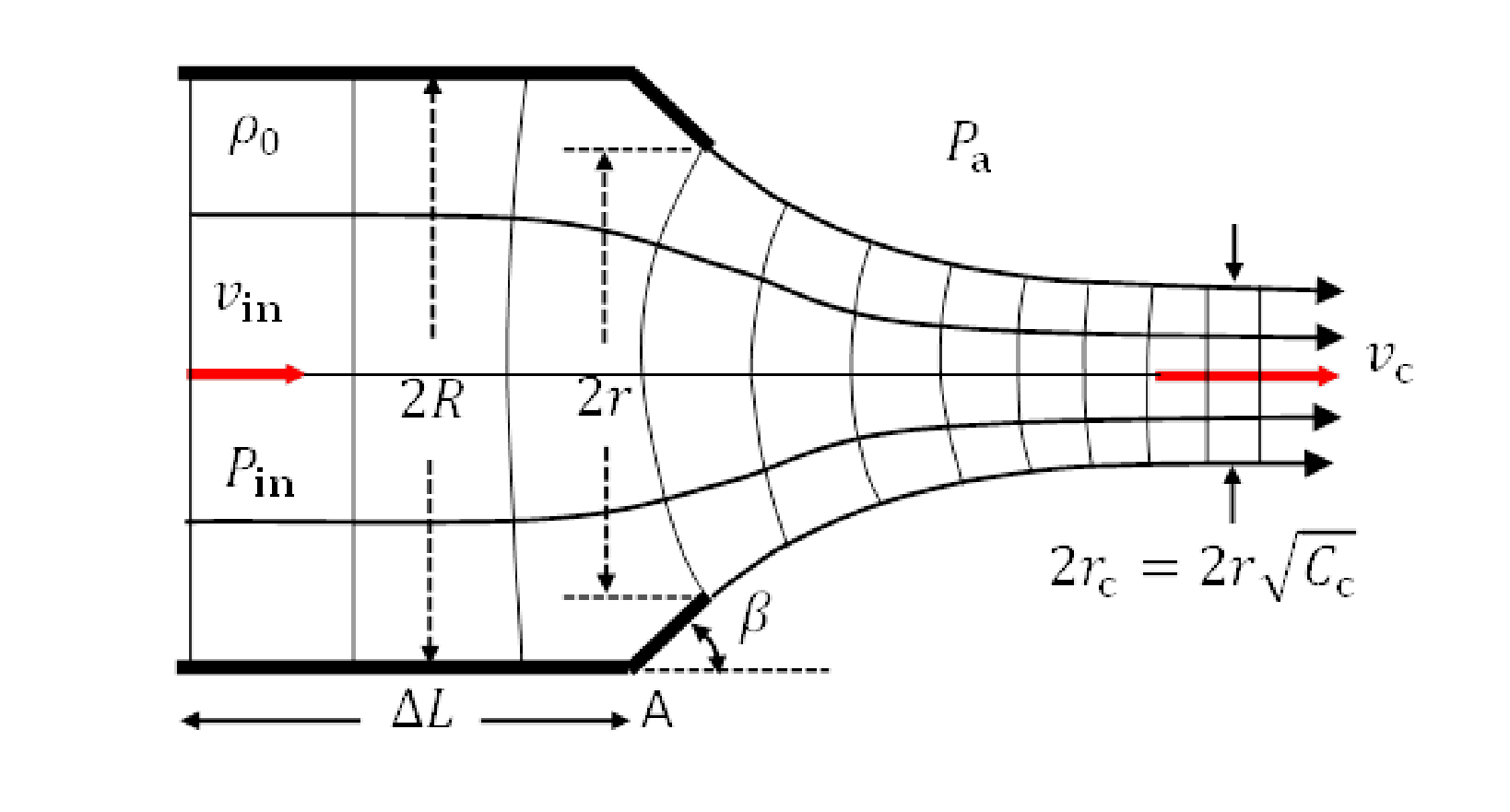
Valve section of length ΔL and inner diameter 2R ending at A, with a cone-shaped outlet of angle β and orifice diameter 2r; inlet quantities ρ0, v_in, P_in on the left; stream lines and normal lines show the jet contracting outside the valve in the atmosphere at P_a to diameter 2r_c = 2r√C_c with velocity v_c. — Fig. 2: Valve dimensions and contraction of jet.

It is known that, after leaving the valve into the atmosphere, the cross section of the flow will contract until it reaches a minimum where the stream lines are again parallel. At this point of minimum, the flow velocity is $v_\mathrm{c}$ and the cross section of the flow has a radius $r_\mathrm{c} = r\sqrt{C_\mathrm{c}}$ . Here $C_\mathrm{c}$ , called the contraction coefficient, depends on the ratio $r/R$ and the cone angle $\beta$ as shown in Table 1.

$r/R$	$C_\mathrm{c}(\beta = 45^{\circ})$	$C_\mathrm{c}(\beta = 90^{\circ})$
0.00	0.746	0.611
0.20	0.747	0.616
0.30	0.748	0.622
0.40	0.749	0.631
1.00	1.000	1.000

Table 1. Contraction Coefficients for Orifices

B.1 Find the excess pressure $\Delta P_\mathrm{in} = P_\mathrm{in} - P_\mathrm{a}$ at the valve inlet where the stream lines are parallel. Give your answer in terms of $\rho_0$ , $v_\mathrm{in}$ , $r$ , $R$ , and $C_\mathrm{c}$ . [1 т.]

For all tasks in Part C and Part D, we consider the reservoir-pipe system in Fig. 1 and make the following assumptions:

Speed of propagation $c$ and density $\rho_0$ of liquid are given constants independent of flow velocity. The ambient atmospheric pressure $P_\mathrm{a}$ and the acceleration of gravity $g$ are constant.
Initially, the valve is fully open and the flow in the pipe is steady with fluid pressure $P_0$ and velocity $v_0$ .
As in Fig. 1 and Fig. 2, the pipe has length $L$ and radius $R$ . The valve T is a circular opening of variable radius $r$ with angle $\beta = 90^{\circ}$ and its length $\Delta L$ is negligible so that the valve inlet is effectively at the end A of the pipe. Effects of gravity on the efflux are negligible.
Liquid in the reservoir is quasi-static so that its pressure $P_h$ near the pipe entrance B remains constant and we assume that the variation of fluid pressure across the pipe is negligible so that the flow is one-dimensional throughout the pipe.
The model outlined in Part B may be used to determine the excess pressure $\Delta P_\mathrm{in} = P_\mathrm{in} - P_\mathrm{a}$ at the valve inlet.

Part C. Water-Hammer Effect due to Fast Closure of Flow Control Valve (1.8 points)

Refer to the reservoir-pipe system in Fig. 1. When liquid flow in the pipe is obstructed by complete or partial closure of the valve, a pressure wave starts traveling upstream. It gets reflected at the reservoir end of the pipe and travels back to the valve and gets reflected there. Then another pressure wave is generated and the process just described is repeated. This causes a sequence of sudden pressure surges and dips for liquid element next to the valve and is referred to as water-hammering.

C.1 Refer to Fig. 1 and Fig. 2. Find the pressure $P_0$ and velocity $v_0$ of the steady flow in the pipe when valve T is fully open ( $r = R$ ). Give answers in terms of $\rho_0$ , $g$ , $h$ , and $P_\mathrm{a}$ . [0,6 т.]

C.2 Consider the same steady flow as in task C.1 with pressure $P_0$ and flow velocity $v_0$ . Now, at $t = 0$ , the valve is closed ( $r = 0$ ) instantly. A pressure wave heads toward the reservoir with speed of propagation $c$ . Take note $P_h = P_0 + \rho_0 g h$ . Let $\tau = 2L/c$ . What are the fluid pressure $P(t)$ and flow velocity $v(t)$ in the pipe when $t$ is getting very close to each of the instants $\tau/2$ and $\tau$ ? [1,2 т.]

Part D. Water-Hammer Effect due to Slow Closure of Flow Control Valve (5.0 points)

Consider again the same steady flow as in task C.1 with pressure $P_0$ and flow velocity $v_0$ . Now we close the valve slowly and adopt a finite-step approach to simulate the closing process.

Starting at time $t = 0$ , the instant reduction of the radius $r$ of the valve (see Fig. 2) is carried out sequentially at a time interval $\tau = 2L/c$ . Immediately after each instant reduction of radius, the flow in the valve region is approximated to be steady as in Part B. The pressure and velocity at the valve are then different from those of the rest of the flow in the pipe.

For each closing step $n$ , its duration and the radius $r_n$ of the valve opening are specified in Table 2 along with the symbols used to represent the corresponding fluid pressure $P_n$ and flow velocity $v_n$ at the valve.

closing step $n$	time interval of step $n$	ratio $r_n/R$	pressure at valve when $t = (n-1)\tau$	flow velocity at valve when $t = (n-1)\tau$
$n = 0$	$t < 0$	$1.00$	$P_0$	$v_0$
$n = 1$	$0 \le t < \tau$	$0.40$	$P_1$	$v_1$
$n = 2$	$\tau \le t < 2\tau$	$0.30$	$P_2$	$v_2$
$n = 3$	$2\tau \le t < 3\tau$	$0.20$	$P_3$	$v_3$
$n = 4$	$3\tau \le t < 4\tau$	$0.00$	$P_4$	$v_4 = 0$

Table 2. Valve closing steps

Take fluid density $\rho_0$ and speed of propagation $c$ as constants. Let $n = 0, 1, 2, 3, 4$ . Define $\Delta P_n = P_n - P_0$ and $\Delta v_n = v_n - v_0$ . Make sure to enforce the approximation $P_h = P_0$ .

D.1 Obtain an equation which expresses $\Delta P_n/(\rho_0 c)$ in terms of $\Delta P_{n-1}/(\rho_0 c)$ , $v_{n-1}$ , and $v_n$ . It must be valid for all steps $n > 0$ specified in Table 2. For $n = 1, 2, 3$ , obtain also an equation which allows $v_n$ to be computed if both $v_{n-1}$ and $\Delta P_{n-1}/(\rho_0 c)$ are known. [3 т.]

D.2 Apply the result of task D.1 to water flow with $v_0 = 4.0\ \mathrm{m/s}$ . Use the graph paper provided in the Answer Sheet to make all plots of $\Delta P$ versus $\rho_0 c v$ . Be sure to draw lines and curves intersecting at points having coordinates which give the values of $\rho_0 c v_n$ and $\Delta P_n$ for steps $n = 1, 2, 3, 4$ . On the plot, label each point of intersection $(\rho_0 c v_n, \Delta P_n)$ with the value of $n$ to which it corresponds. From the graph, estimate values of $\rho_0 c v_n$ and $\Delta P_n$ (both in units of MPa) for $n = 1, 2, 3, 4$ . [2 т.]

Отговори

Решение

Solution

Water Hammer

Part A. Excess Pressure and Propagation of Pressure wave

Reservoir at P_a feeding a pipe from B to A with valve T; the shaded region next to the closed valve holds liquid with ρ1, P1 and velocity v1 pointing left, bounded by the wave front moving left with speed c; ahead of it the liquid has ρ0, P0 and velocity v0 to the right; axis x points right. — Fig. S1. Pressure wave (shaded) with speed $c$

A.1 (1.6 pt) Excess pressure and speed of propagation of the pressure wave

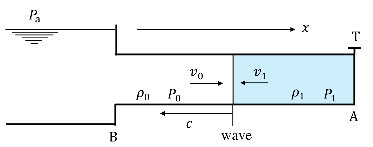
When the valve opening is suddenly blocked, fluid pressure at the valve jumps from $P_0$ to $P_1 = P_0 + \Delta P_\mathrm{s}$ , thus sending a pressure wave traveling upstream (to the left) with speed $c$ and amplitude $\Delta P_\mathrm{s}$ . Taking positive $x$ direction as pointing to the right, the velocity of fluid particles next to the valve changes from $v_0$ to $v_1$ ( $v_1 \le 0$ ). Thus the velocity change is $\Delta v = v_1 - v_0$ .

In a frame moving to left (along $-x$ direction) with speed $c$ , i.e., riding on the wave (see Fig. S1), velocity of fluid in the pressure wave is $c + v_1$ , while that of the incoming fluid in the steady flow ahead of the wave is $c + v_0$ . Let $\rho_1$ be the density of fluid in the pressure wave. From conservation of mass, i.e., equation of continuity, we have

\rho_0(c + v_0) = \rho_1(c + v_1) \qquad (a1)

or, by letting $\Delta\rho \equiv \rho_1 - \rho_0$ ,

\frac{\Delta\rho}{\rho_1} = 1 - \frac{\rho_0}{\rho_1} = \frac{v_0 - v_1}{c + v_0} = \frac{-\Delta v}{c + v_0} \qquad (a2)

Moreover, impulse imparted to the fluid must equal its momentum change. Thus, in a short time interval $\tau$ after the valve is closed, we must have

\rho_0(c + v_0)\tau[(c + v_1) - (c + v_0)] = -\tau\Delta P = (P_0 - P_1)\tau \qquad (a3)

\Delta P_\mathrm{s} = -\rho_0 c\left(1 + \frac{v_0}{c}\right)(v_1 - v_0) = -\rho_0 c\left(1 + \frac{v_0}{c}\right)\Delta v \quad\Rightarrow\quad \alpha = -\left(1 + \frac{v_0}{c}\right) \qquad (a4)

If $v_0/c \ll 1$ , we have

\Delta P_\mathrm{s} = -\rho_0 c\Delta v \qquad (a5)

Note that the negative sign in Eqs. (a4) and (a5) follows from the fact that the direction of propagation is opposite to the positive direction for $x$ axis (and velocity). Otherwise the sign should be positive. Note also that for a compressional wave ( $\Delta P_\mathrm{s} > 0$ ), the velocity imparted to the fluid particle is in the direction of propagation, while for an extensional wave ( $\Delta P_\mathrm{s} < 0$ ), the velocity imparted is in the opposite direction of propagation.

Eqs. (a2) and (a4) can be combined to give

\Delta P_\mathrm{s} = \rho_0 c^2\left(1 + \frac{v_0}{c}\right)^2\frac{\Delta\rho}{\rho_1} \qquad (a6)

From the definition of the bulk modulus $B$ , which is assumed to be constant, it follows

\Delta P_\mathrm{s} = B\,\frac{V_0 - V_1}{V_0} = B\,\frac{1/\rho_0 - 1/\rho_1}{1/\rho_0} = B\,\frac{\Delta\rho}{\rho_1} \qquad (a7)

From Eqs. (a6) and (a7), we obtain

\rho_0 c^2\left(1 + \frac{v_0}{c}\right)^2 = B \qquad (a8)

Thus

c = \sqrt{\frac{B}{\rho_0}} - v_0 \qquad\Rightarrow\qquad \gamma = 1 \qquad \beta = -v_0 \qquad (a9)

However, if in the definition of bulk modulus one uses the fractional change of density $\Delta\rho/\rho_0$ instead of $-\Delta V/V_0$ , the result is then $\gamma = 1 + \Delta P_\mathrm{s}/B$ .* Either result is considered valid.

If $v_0/c \ll 1$ , we have

c = \sqrt{\frac{B}{\rho_0}} \qquad (a10)

*The result (a7) is pointed out by Dr. Jaan Kalda.

A.2 (0.6 pt) Values of $c$ and $\Delta P_\mathrm{s}$ for water flow

Ans:

From Eqs. (a5) and (a10), we have

c = \sqrt{B/\rho_0}

\Delta P_\mathrm{s} = \rho_0 c v_0 = v_0\sqrt{\rho_0 B}

Putting in the given values $v_0 = 4.0\ \mathrm{m/s}$ , $v_1 = 0$ , $\rho_0 = 1.0\times 10^3\ \mathrm{kg/m^3}$ , and $B = 2.2\times 10^9\ \mathrm{Pa}$ , we have

c = \sqrt{B/\rho_0} = 1.5\times 10^3\ \mathrm{m/s} \qquad (b1)

\Delta P_\mathrm{s} = v_0\sqrt{\rho_0 B} = 5.9\ \mathrm{MPa} \qquad (b2)

so that $\Delta P_\mathrm{s}$ is nearly 59 times the standard pressure.

Note that $v_0/c \sim 10^{-3}$ so that the use of approximate formulas (a5) and (a10) is justified when solving tasks in this problem.

Part B. A Model for the Flow-Control Valve

(B.1) (1.0 pt) Excess pressure at valve inlet

The valve of Fig. 2 redrawn with the valve walls in red: section of length ΔL and diameter 2R ending at A, cone outlet of angle β and orifice diameter 2r, inlet quantities ρ0, v_in, P_in, and the contracted jet at P_a with diameter 2r_c = 2r√C_c and velocity v_c. — Fig. 2. Valve dimensions and contraction of jet.

Ans:

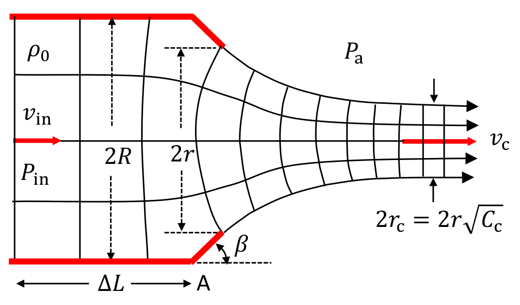
The model assumes the fluid to be incompressible. Neglecting effects of gravity, Bernoulli’s principle gives us

\tfrac{1}{2}\rho_0 v_\mathrm{in}^2 + P_\mathrm{in} = \tfrac{1}{2}\rho_0 v_\mathrm{c}^2 + P_\mathrm{a} \qquad (c1)

Equation of continuity and definition of contraction coefficient imply that

\pi R^2 v_\mathrm{in} = \pi r_\mathrm{c}^2 v_\mathrm{c} = \pi r^2 C_\mathrm{c} v_\mathrm{c}

Therefore

v_\mathrm{c} = \frac{1}{C_\mathrm{c}}\left(\frac{R}{r}\right)^2 v_\mathrm{in} \qquad (c2)

From Eqs. (c1) and (c2), we obtain

\Delta P_\mathrm{in} = P_\mathrm{in} - P_\mathrm{a} = \frac{1}{2}\rho_0 v_\mathrm{in}^2\left[\frac{1}{C_\mathrm{c}^2}\left(\frac{R}{r}\right)^4 - 1\right] = \frac{k}{2}\rho_0 v_\mathrm{in}^2 \qquad (c3)

This may be cast into a form involving only dimensionless variables:

\frac{\Delta P_\mathrm{in}}{\rho_0 c^2} = \frac{1}{2}\left(\frac{v_\mathrm{in}}{c}\right)^2\left[\frac{1}{C_\mathrm{c}^2}\left(\frac{R}{r}\right)^4 - 1\right] = \frac{k}{2}\left(\frac{v_\mathrm{in}}{c}\right)^2 \qquad (c4)

where

k = \left[\frac{1}{C_\mathrm{c}^2}\left(\frac{R}{r}\right)^4 - 1\right] \qquad (c5)

Thus we see from eq. (c4) that $\Delta P_\mathrm{in}$ is a quadratic function of $v_\mathrm{in}$ .

Part C. Water-Hammer Effect due to Fast Closure of Flow-Control Valve

(C.1) (0.6 pt) Pressure $P_0$ and velocity $v_0$ when the valve is fully open

Ans:

According to Bernoulli’s theorem and the definition of $P_h$ , we have

\tfrac{1}{2}\rho_0 v_0^2 + P_0 = \tfrac{1}{2}\rho_0 v_\mathrm{c}^2 + P_\mathrm{a} = 0 + P_\mathrm{a} + \rho_0 g h = P_h \qquad (d1)

From the second equality in the preceding equation, it follows

v_\mathrm{c} = \sqrt{2gh}

Furthermore, from continuity equation and $C_\mathrm{c}(r = R) = 1.0$ , we have

\pi R^2 v_0 = \pi(C_\mathrm{c}R)^2 v_\mathrm{c} = \pi R^2 v_\mathrm{c} \;\Rightarrow\; v_0 = v_\mathrm{c} = \sqrt{2gh} \qquad (d2)

Therefore

P_0 = P_\mathrm{a} = P_h - \rho_0 g h \qquad (d3)

(C.2) (1.2 pt) Pressure $P(t)$ and flow velocity $v(t)$ just before $t = \frac{\tau}{2} = \frac{L}{c}$ and $t = \tau$

Ans:

When the valve is open, the flow in the pipe is steady with velocity $v_0$ and pressure $P_0$ . The sudden closure of the valve causes an excess pressure $\Delta P_s$ on the fluid element next to the valve, causing it to stop with velocity $v_1 = 0$ . The velocity change is thus $\Delta v = v_1 - v_0 = -v_0$ . Thus, according to Eq. (a5), the excess pressure on the fluid is given by

\Delta P_\mathrm{s} = -\rho_0 c\Delta v = \rho_0 c v_0 \qquad (e1)

At time $t = \tau/2 = L/c$ , the pressure wave reaches the reservoir. The velocity of fluid in the length of the pipe has all changed to $v(\tau/2) = v_1 = v_0 + \Delta v = 0$ and the fluid pressure is $P(\tau/2) = P_1 = P_0 + \Delta P_\mathrm{s} = P_0 + \rho_0 c v_0$ .

At the reservoir end of the pipe, fluid pressure reduces to the constant hydrostatic pressure $P_h = P_0 + \rho_0 g h$ . Equivalently, we may say that the reservoir acts as a free end for the pressure wave and, in reducing its excess pressure to $P_h$ , causes a compression wave to be reflected as an expansion wave. Relative to the hydrostatic pressure $P_h$ , the amplitude of the incoming pressure wave is $\Delta P_\mathrm{1r} = P_1 - P_h$ , hence the reflected expansion wave will have an amplitude $\Delta P_1' = -\Delta P_\mathrm{1r}$ and we have

\Delta P_1' = -\Delta P_\mathrm{1r} = P_h - P_1 = (P_0 + \rho_0 g h) - (P_0 + \rho_0 c v_0) = -\rho_0 c(v_0 - gh/c) \qquad (e2)

(Here we allow the pressure amplitude to have both signs with negative amplitude signifying an expansion wave.) This will cause the fluid at the reservoir end of the pipe to suffer a velocity change (keeping in mind that the direction of propagation is now the same as the $+x$ axis)

\Delta v_\mathrm{1r} = +\Delta P_1'/(\rho_0 c) = -(v_0 - gh/c)

Consequently, its velocity changes to

v_\mathrm{1r} = v_1 + \Delta v_\mathrm{1r} = 0 - \left(v_0 - \frac{gh}{c}\right) \qquad (e3)

Ahead of the front of the reflected wave, conditions are unchanged and the particle velocity is still $v_1 = 0$ and the fluid pressure is still $P_1 = P_0 + \Delta P_\mathrm{s}$ , but behind the wave front the particle velocity now becomes $v_\mathrm{1r} = -(v_0 - gh/c)$ and the pressure becomes

P_1 + \Delta P_1' = (P_0 + \rho_0 c v_0) - \rho_0 c\left(v_0 - \frac{gh}{c}\right) = P_0 + \rho_0 g h \qquad (e4)

Therefore, just moment before $t = \tau = 2L/c$ when the front of the reflected wave reaches the valve, the fluid in the whole length of the pipe will be under the pressure $P(\tau) = P_0 + \rho_0 g h = P_h$ as given in Eq. (e4) , and all fluid particles in the pipe will move, as given in Eq. (e3), with velocity $v(\tau) = v_\mathrm{1r} = -v_0 + gh/c$ , i.e., the fluid in the pipe is expanding and flowing toward the reservoir.

Part D. Water-Hammer Effect due to Slow Closure of Flow-Control Valve

(D.1) (3.0 pt) Recursion relations for $\Delta P_n$ and $v_n$

Ans:

Enforcing the approximation $P_h = P_0 + \rho_0 g h \approx P_0$ is equivalent to putting $h = 0$ in all of the results obtained in task (e).

(1) Partial closing $n = 1$

At the valve, immediately after partial closing $n = 1$ , fluid pressure jumps from $P_0$ to $P_1$ , causing flow velocity to change from $v_0$ to $v_1$ . The pressure and velocity changes are related by Eq. (a5):

\frac{1}{\rho_0 c}(P_1 - P_0) = -(v_1 - v_0) \qquad (f1)

Just before reflection by the reservoir, the fluid in the entire pipe has pressure $P_1$ and velocity $v_1$ . After reflection by the reservoir, i.e., a free end, and before the start of valve closure $n = 2$ , the fluid in the entire pipe has pressure (Eq. (e4) with $h = 0$ )

P_1 - (P_1 - P_0) = P_0

and velocity

v_1' = v_1 + \frac{-(P_1 - P_0)}{\rho_0 c} = v_1 + (v_1 - v_0)

(2) Partial closing $n = 2$

Immediately after partial closing $n = 2$ , valve pressure changes from $P_0$ to $P_2$ , causing flow velocity to change from $v_1'$ to $v_2$ . The pressure and velocity changes are given by Eq. (a5):

\frac{1}{\rho_0 c}(P_2 - P_0) = -(v_2 - v_1') = -v_2 + v_1 + (v_1 - v_0) \qquad (f2)

Using Eq. (f1), we may rewrite the preceding equation as

\frac{1}{\rho_0 c}(P_2 - P_0) = -(v_2 - v_1) - \frac{1}{\rho_0 c}(P_1 - P_0) \qquad (f3)

Just before reflection by the reservoir, the fluid in the entire pipe has pressure $P_2$ and velocity $v_2$ . After reflection by the reservoir and before valve closure $n = 3$ , the fluid in the entire pipe has pressure

P_2 - (P_2 - P_0) = P_0

and velocity

v_2' = v_2 + (v_2 - v_1')

(3) Partial closing $n = 3$

Immediately after partial closing $n = 3$ , valve pressure changes from $P_0$ to $P_3$ , causing flow velocity to change from $v_2'$ to $v_3$ . The pressure and velocity changes are given by Eq. (a5):

\frac{1}{\rho_0 c}(P_3 - P_0) = -(v_3 - v_2') = -v_3 + v_2 + (v_2 - v_1') \qquad (f4)

Using Eq. (f2), we may rewrite the preceding equation as

\frac{1}{\rho_0 c}(P_3 - P_0) = -(v_3 - v_2) - \frac{1}{\rho_0 c}(P_2 - P_0) \qquad (f5)

Just before reflection by the reservoir, the fluid in the entire pipe has pressure $P_3$ and velocity $v_3$ . After reflection by the reservoir and before valve closure $n = 4$ , the fluid in the entire pipe has pressure

P_3 - (P_3 - P_0) = P_0

and velocity

v_3' = v_3 + (v_3 - v_2')

(4) Partial closing $n = 4$

When the valve is fully shut at valve closing $n = 4$ , the valve becomes a fixed end, so the fluid velocity at the valve changes from $v_3'$ to $v_4 = 0$ . The pressure $P_4$ at the valve is then given by Eq. (a5):

\frac{1}{\rho_0 c}(P_4 - P_0) = -(v_4 - v_3') = -v_4 + v_3 - \frac{1}{\rho_0 c}(P_3 - P_0) \qquad (f6)

Finally, if we take note of the fact that $\Delta P_0 = 0$ and $v_4 = 0$ , then all equations obtained above relating excess pressures and velocity changes after valve closings all have the same form:

\frac{\Delta P_n}{\rho_0 c} = -(v_n - v_{n-1}) - \frac{\Delta P_{n-1}}{\rho_0 c} \qquad (n = 1,2,3,4) \qquad (f7)

To solve for $\Delta P_n = P_n - P_0$ , we note that, from Eqs. (c3) and (c5), we have another relation between $\Delta P_n$ and $v_n$ :

\Delta P_n = \frac{1}{2}k_n\rho_0 {v_n}^2 \qquad (n = 1,2,3) \qquad (f8)

where $C_n$ represents $C_\mathrm{c}$ for $r = r_n$ and

k_n = \left[\frac{1}{C_n^2}\left(\frac{R}{r_n}\right)^4 - 1\right] \qquad (n = 1,2,3) \qquad (f9)

Combining Eqs. (f7) and (f8), we have a quadratic equation for $v_n$ :

\frac{1}{2}k_n\left(\frac{v_n}{c}\right)^2 + \frac{v_n}{c} + \left(\frac{\Delta P_{n-1}}{\rho_0 c^2} - \frac{v_{n-1}}{c}\right) = 0 \qquad (n = 1,2,3) \qquad (f10)

which can be solved readily using the formula

\frac{v_n}{c} = \frac{-1 + \sqrt{1 + 2k_n\left(\frac{v_{n-1}}{c} - \frac{\Delta P_{n-1}}{\rho c^2}\right)}}{k_n} \qquad (n = 1,2,3) \qquad (f11)

If both $\Delta P_{n-1}/(\rho c^2)$ and $(v_{n-1}/c)$ are known, Eq. (f11) may be used to compute $v_n/c$ and then find $\Delta P_n/(\rho c^2)$ by using Eq. (f8). Therefore, Eq. (f7) may be solved iteratively starting with $n = 1$ until $n = 3$ . For $n = 4$ , we know $v_n = 0$ , so Eq. (f7) may be used directly to find $\Delta P_n$ .

Note that, from Eq. (f8), $\Delta P_{n-1}$ is a quadratic function of $v_{n-1}$ , so that if $v_{n-1}$ is known, then $v_n$ may be computed using Eq. (f11) and then $\Delta P_n$ may again be computed using Eq. (f8).

(D.2) (2.0 pt) Estimating $\Delta P_n$ and $\rho_0 c v_n$ by graphical method

Ans:

To solve Eqs. (f7) and (f8) using graphical method, we rewrite them as follows:

\Delta P_n = -(\rho_0 c v_n - \rho_0 c v_{n-1}) - \Delta P_{n-1} \qquad (n = 1,2,3,4) \qquad (g1)

\Delta P_n = \frac{k_j}{2\rho_0 c^2}(\rho_0 c v_n)^2 \qquad (n = 1,2,3,4) \qquad (g2)

In a plot of $\Delta P$ vs. $\rho_0 c v$ , Eq. (g1) and Eq. (g2) correspond to a line passing through the point $(\rho_0 c v_{n-1}, -\Delta P_{n-1})$ with slope $-1$ and a parabola passing through the origin, respectively. Thus one may readily obtain the solutions for each step of valve closing by locating their points of intersection, starting with $n = 1$ . The result is shown in the following graph.

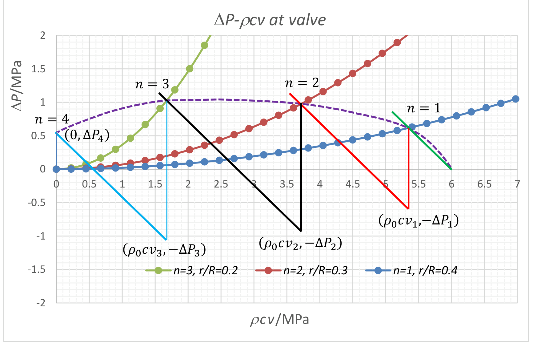
Chart titled 'ΔP-ρcv at valve', ΔP/MPa from -2 to 2 versus ρcv/MPa from 0 to 7: parabolas with markers for n=1, r/R=0.4 (blue), n=2, r/R=0.3 (red) and n=3, r/R=0.2 (green); straight lines of slope -1 from (ρ0cv1, −ΔP1), (ρ0cv2, −ΔP2), (ρ0cv3, −ΔP3) and from 6 on the horizontal axis; intersection points labelled n = 1, n = 2, n = 3 and n = 4 at (0, ΔP4); a dashed purple curve through the intersection points.

Excess Pressures and particle velocities at the valve for slow closing

$n$	$r_n/R$	$C_n$	$k_n$	$v_n/(\mathrm{m/s})$	$\rho_0 c v_n/\mathrm{MPa}$	$\Delta P_n/(\mathrm{MPa})$	$\Delta P_n/(\rho_0 c v_0)$
0	1.00	1.00	0.0	4.0	6.0	0.0	0.0
1	0.40	0.631	97.1	3.6	5.8	0.62	10 %
2	0.30	0.622	318.	2.5	3.8	1.0	17 %
3	0.20	0.616	1646.	1.1	1.7	1.1	18 %
4	0.00			0.0	0.0	0.64	11 %

$\rho_0 c = 1.50\times 10^6\ \mathrm{kg\,m^{-2}\,s^{-1}}$ $\qquad$ $v_0 = 4.0\ \mathrm{m/s}$

Appendix

(The following table and graph are for reference only, not part of the task.)

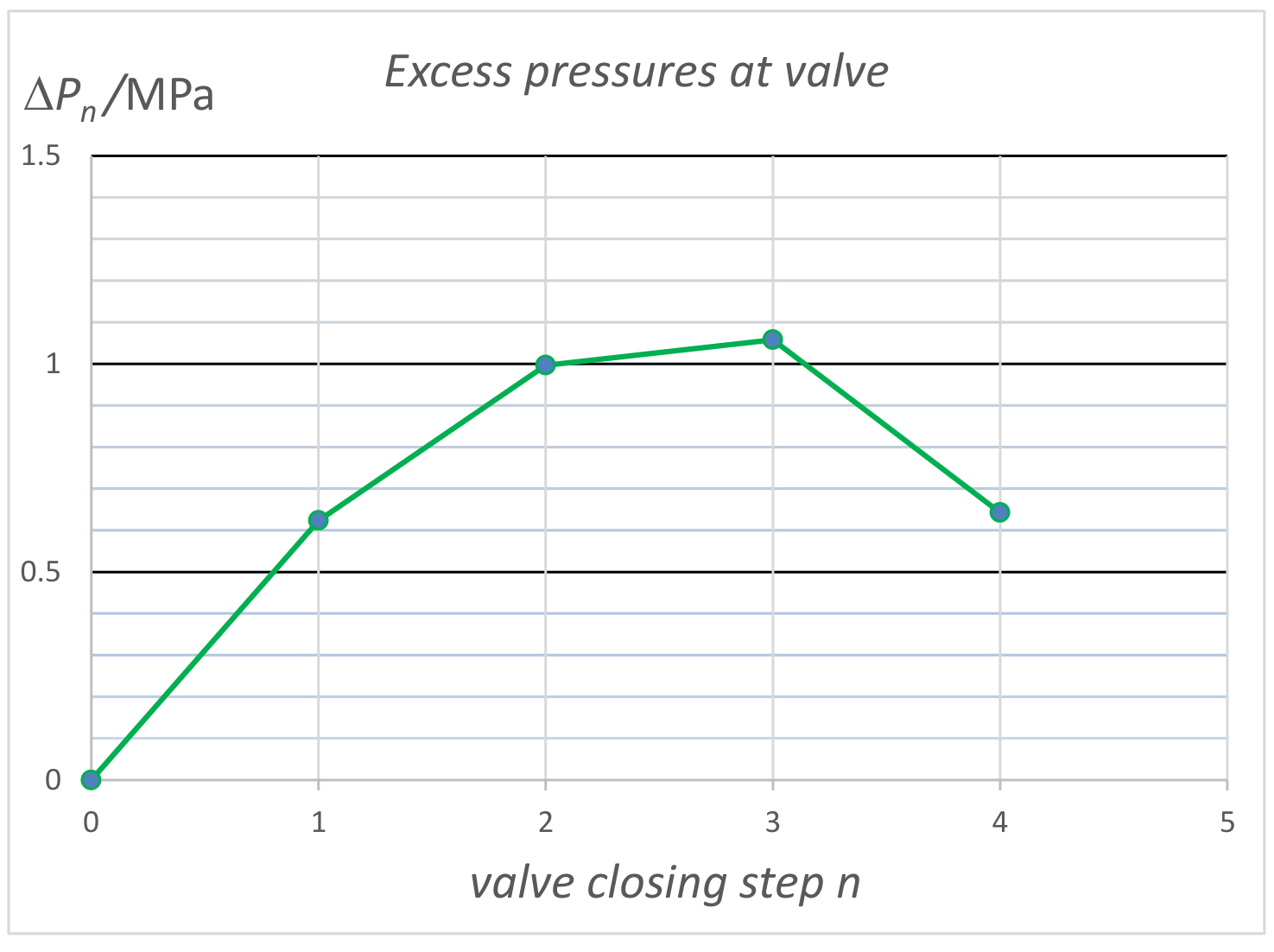
For $v_0 = 4.0\ \mathrm{m/s}$ , $c = 1.5\times 10^3\ \mathrm{m/s}$ , and $\rho = 1.0\times 10^3\ \mathrm{kg/m^3}$ , the results for $v_n$ and $\Delta P_n$ are shown in the following table and graph. They are computed according to equations given in task (f). Note that for a sudden full closure of the valve, we have $\Delta P_\mathrm{sudden} = \rho c v_0 = 6.0\ \mathrm{MPa}$ .

Excess Pressures and particle velocities at the valve for slow closing

$n$	$r_n/R$	$C_n$	$k_n$	$v_n/(\mathrm{m/s})$	$\rho c v_n/\mathrm{MPa}$	$\Delta P_n/(\mathrm{MPa})$	$\Delta P_n/(\rho c v_0)$
0	1.00	1.00	0.0	4.0	6.0	0.0	0.0
1	0.40	0.631	97.1	3.58	5.37	0.624	10 %
2	0.30	0.622	318.	2.50	3.75	0.997	17 %
3	0.20	0.616	1646.	1.13	1.695	1.06	18 %
4	0.00			0.0	0.0	0.643	11 %

Chart titled 'Excess pressures at valve': ΔP_n/MPa from 0 to 1.5 versus valve closing step n from 0 to 5, with points (0, 0), (1, 0.62), (2, 1.0), (3, 1.06), (4, 0.64) joined by a green line.

Оригинал в Архива: Theory Q1 english.pdf · официални решения: Theory Q1 solution.pdf