Съдържание

APhO 2021, Теория — Задача 3. Magnetic Levitation

Оригинал на условието (PDF)Съобщи за грешка

Всички материали от APhO 2021

Theory Q3 — Magnetic Levitation (Asian Physics Olympiad 2021 TAIPEI, English (Official)) · 10 т.

Условие

Useful Information

(1) Directional derivative of a spatial function $f(\vec{r})$ , given by $\vec{\nabla}f(\vec{r})$ , has

$\vec{\nabla}f \equiv (\hat{x}\frac{\partial}{\partial x} + \hat{y}\frac{\partial}{\partial y} + \hat{z}\frac{\partial}{\partial z})f(\vec{r})$ , where $\frac{\partial}{\partial x}f(\vec{r})$ denotes a partial derivative of $f(\vec{r})$ with respect to $x$ while keeping $y$ and $z$ unchanged.

(2) Integral:

$\int_0^{\infty} dt\,\frac{(a+pt)}{[(a+pt)^2+(b+qt)^2]^{3/2}} = \frac{1}{bp-aq}(\frac{b}{\sqrt{a^2+b^2}} - \frac{q}{\sqrt{p^2+q^2}})$ .

Introduction

We intend to study the motion of a small magnetic dipole in the vicinity of a conducting thin film. In the problem text, the terms dipole and monopole are to be regarded, respectively, as synonymous with magnetic dipole and magnetic monopole.

A dipole consisting of a spherical permanent magnet with a uniform magnetization $\vec{M}$ (magnetic dipole moment per unit volume) and a uniform mass density $\rho_0$ may be treated as a point-like object when its radius $R$ is small. Such a dipole representation is good for describing the magnetic field that the dipole produces everywhere outside of its sphere. The representation is also a good approximation for the force acting on the dipole from an applied magnetic field, whenever distances of field sources from the dipole are much larger than $R$ .

A point-like dipole can be considered as a pair of monopoles carrying negative and positive magnetic charges $-q_{\mathrm{m}}$ and $q_{\mathrm{m}}$ respectively. The pair has a vanishingly small separation, but possesses a finite magnetic dipole moment $\vec{m} = q_{\mathrm{m}}\vec{\delta}_{\mathrm{m}}$ . Here $\vec{\delta}_{\mathrm{m}}$ is the displacement vector from the south monopole $(-q_{\mathrm{m}})$ to the north monopole $(+q_{\mathrm{m}})$ . The position of the point-like dipole is chosen to be that of the north monopole.

The magnetic field $\vec{B}_{\mathrm{mp}}$ from a monopole $q_{\mathrm{m}}$ is assumed to have a Coulombic form, given by

\vec{B}_{\mathrm{mp}} = \frac{\mu_0 q_{\mathrm{m}}}{4\pi r^2}\,\hat{r}, \qquad (1)

where $\vec{r}$ is the displacement vector from $q_{\mathrm{m}}$ to the observation point (or field point), $\hat{r}$ is the unit vector $\hat{r} = \vec{r}/r$ , and $\mu_0$ is the free-space permeability. The force exerted by an applied magnetic field $\vec{B}'$ on $q_{\mathrm{m}}$ is given by $\vec{F} = q_{\mathrm{m}}\vec{B}'$ . It follows, from extending the concept of the monopole field just described in Eq.(1), that the magnetic field $\vec{B}$ from a point-dipole is derivable from a scalar potential $\Phi$ , given by the form $\vec{B} = -\vec{\nabla}\Phi$ . The scalar potential $\Phi$ is also called the magnetic potential.

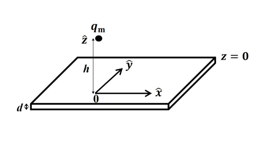
The conducting thin film is uniform with thickness $d$ in the $z$ direction (Fig. 1). It extends horizontally in $x$ and $y$ directions to infinity and its upper surface is located at a distance $h$ from either a point monopole or a dipole. We consider only the case $h \gg d$ . This allows us to take the electric current density induced in the film to be independent of $z$ . We also assume that the displacement current effect to be negligible.

Perspective drawing of a thin flat slab of thickness d. The origin 0 is on its upper surface (labelled z = 0), with unit vectors x-hat and y-hat drawn in the plane and z-hat pointing up; the monopole q_m is a black dot on the z axis at height h above the origin. — Fig.1 A monopole $q_{\mathrm{m}}$ appears at a distance $h$ from a conducting thin film of thickness $d$ . The origin of the coordinates is located on the upper surface.

The problem is divided into three parts. In Part A, the system consists of a monopole and a thin film, while in Parts B and C, a moving dipole and a thin film.

We choose the $z = 0$ plane to coincide with the upper surface of the thin film. The vector $\vec{\rho} = x\hat{x} + y\hat{y} = \rho\hat{\rho}$ denotes the in-plane position vector.

Part A. Sudden appearance of a magnetic monopole: initial response and subsequent time evolution of the response in the thin film (3.0 points)

We first focus on the initial response of the conducting thin film when at time $t = 0$ a north monopole $q_{\mathrm{m}}$ appears suddenly at the position $\vec{r}_{\mathrm{mp}} = h\hat{z}\ (h > 0)$ , as is shown in Fig. 1. The monopole remains stationary in all later times ( $t > 0$ ).

Our interest here is the initial total magnetic field $\vec{B}(\vec{\rho}, z)$ in regions $z \ge 0$ and $z \le -d$ , and the induced electric current density in the thin film. The total magnetic field $\vec{B} = \vec{B}_{\mathrm{mp}} + \vec{B}'$ , where magnetic fields $\vec{B}_{\mathrm{mp}}$ and $\vec{B}'$ are, respectively, due to the monopole and the induced current in the thin film. The initial $\vec{B}(\vec{\rho}, z)$ we refer to is at the time $t_0$ , which falls within the interval $h/c \le t_0 \ll \tau_{\mathrm{c}}$ . Here $\tau_{\mathrm{c}}$ is a time constant characterizing the subsequent response of the thin film, and $c$ is the speed of light in vacuum. In this problem, we take the limit $h/c \to 0$ and hence let $t_0 = 0$ .

The calculation of the initial total magnetic field $\vec{B}(\vec{\rho}, z)$ (at $t_0 = 0$ ) is facilitated by introducing an image monopole. For $\vec{B}(\vec{\rho}, z)$ in the region $z \ge 0$ , the image monopole has a magnetic charge $q_{\mathrm{m}}$ and is located at $z = -h$ . On the other hand, for $\vec{B}(\vec{\rho}, z)$ in the region $z \le -d$ , the image monopole has a magnetic charge $-q_{\mathrm{m}}$ and is located at $z = h$ .

Initial response

A.1 Obtain the initial total magnetic field $\vec{B}(\vec{\rho}, z)$ in $z \ge 0$ at $t_0 = 0$ . [0,4 т.]

A.2 Obtain the initial total magnetic field $\vec{B}(\vec{\rho}, z)$ in $z \le -d$ at $t_0 = 0$ . [0,2 т.]

A.3 Find the initial magnetic flux $\Phi_{\mathrm{B}}$ through surfaces at $z = 0$ , and at $z = -d$ . [0,4 т.]

A.4 Obtain the initial induced electric current density $\vec{j}(\vec{\rho})$ in the conducting thin film at $t_0 = 0$ . [0,6 т.]

For $t > 0$ , the total magnetic field $\vec{B}$ becomes $\vec{B}(\vec{\rho}, z; t) = \vec{B}_{\mathrm{mp}}(\vec{\rho}, z) + \vec{B}'(\vec{\rho}, z; t)$ , by superposition, with $\vec{B}'(\vec{\rho}, z; t)$ due to the induced electric current in the thin film. You are required below to obtain an equation for $B_z'(\rho, z; t)$ near the $z = 0$ thin film surface. The time-evolution behavior of $B_z'$ would reveal a moving image-monopole picture for the description of the $\vec{B}'$ field near $z \approx 0$ in $t > 0$ .

The equation for $B_z'$ inside the thin film is given below,

\frac{\partial^2 B_z'(\rho, z; t)}{\partial z^2} = \mu_0\sigma\frac{\partial B_z'(\rho, z; t)}{\partial t}. \qquad (2)

This equation has been obtained from imposing inside the thin film the Maxwell equation and the Ohmic behavior of the conducting thin film ( $\vec{j} = \sigma\vec{E}$ , where $\sigma$ is the electrical conductivity) while neglecting the displacement-current effect. Term being neglected on the left-hand side of Eq.(2) is $\frac{1}{\rho}\frac{\partial}{\partial\rho}(\rho\frac{\partial B_z'}{\partial\rho})$ , based on the $h \gg d$ condition.

Subsequent response

A.5 Obtain from Eq. (2) an equation of $B_z'(\rho, z; t)$ near $z \approx 0$ . The equation contains first partial derivatives of $B_z'(\rho, z; t)$ with respect to $z$ , and, separately, to $t$ . [0,6 т.]

A.6 Solve for the general form of $B_z'(\rho, z; t)$ near $z \approx 0$ in $t > 0$ . [0,4 т.]

A.7 Show that your solution in A.6 reveals a moving image-monopole picture for the magnetic field $B_z'(\rho, z \approx 0; t)$ , with a downwardly moving velocity. Find the speed $v_0$ of the image monopole in terms of known parameters from the problem text. [0,4 т.]

Part B. Magnetic force acting on a point-like dipole moving with a constant velocity and at a constant h (4.0 points)

The moving image-monopole concept developed in A.7 for $B_z'$ near $z \approx 0$ can be assumed to hold also for the $\vec{B}'$ field in the $z \ge 0$ region. This assumption is good as long as the time evolution is sufficiently slow in the conducting thin film response.

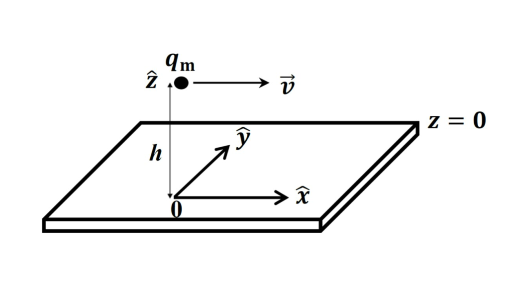
The same slab with origin 0 on its upper surface (z = 0), axes x-hat, y-hat and z-hat; the monopole q_m sits at height h above the origin with an arrow v pointing in the +x direction. — Fig. 2 A monopole $q_{\mathrm{m}}$ moves with a constant velocity $\vec{v}$ and a constant height $h$ from the conducting thin film. As shown are its coordinates at $t = 0$ .

A monopole $q_{\mathrm{m}}$ (Fig. 2) is caused to move in a constant velocity $v\hat{x}$ , with $v \ll c$ , and a constant height, at $z = h$ , motion up to the present moment ( $t = 0$ ). Its present coordinates $(x, y)$ are $(0, 0)$ . Our focus is on the magnetic potential $\Phi_+$ due to all image monopoles generated by this moving monopole along its trajectory.

By splitting $q_{\mathrm{m}}$ 's trajectory into discrete time steps (a very small time step $\tau$ ), we replace the motion of the $q_{\mathrm{m}}$ by a hopping at the beginning moment of each time step. The hopping is represented by a simultaneous removal and creation of the monopoles. The position of the created monopole coincides with a point on its trajectory right at the beginning moment of this time step. Thus the position of the removed monopole coincides with its trajectory position at the beginning moment of the previous time step. This is achieved by a simultaneous sudden appearance of two magnetic monopoles: $q_{\mathrm{m}}$ and $-q_{\mathrm{m}}$ at, respectively, the trajectory positions corresponding to the beginning moments of this and the previous time step. The two positions are separated by a hopping distance $\Delta x = v\tau$ . This time-step approach facilitates the determination of all the image magnetic monopoles, and their positions, that are generated in all the time steps.

A moving monopole

B.1 Write down the present $(t = 0)$ positions of all the image monopoles of the types $q_{\mathrm{m}}$ and $-q_{\mathrm{m}}$ . The beginning moments of the time steps are at $t = -n\tau$ , where $n \ge 0$ . [0,8 т.]

B.2 Find the summation form of the magnetic potential $\Phi_+(x, z)$ at $t = 0$ from all the image monopoles in B.1. Calculate $\Phi_+(x, z)$ . [0,7 т.]

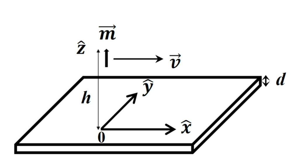
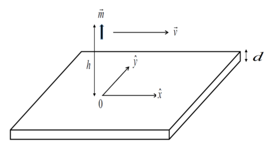
The slab of thickness d with origin 0 on its upper surface and axes x-hat, y-hat, z-hat; at height h above the origin a short upward arrow marks the dipole moment m, with a horizontal arrow v pointing in the +x direction. — Fig. 3 A dipole with an **upward-pointing** magnetic dipole moment $\vec{m}$ moves with a constant $\vec{v}$ and a constant height $h$ from the conducting thin film. As shown are its coordinates at $t = 0$ .

Now consider a point-like moving magnetic dipole as shown in Fig. 3. The dipole, with a dipole moment $\vec{m} = m\hat{z}$ , is caused to move in a constant velocity $v\hat{x}$ , and a constant height ( $z = h$ ) motion up to the present moment ( $t = 0$ ), where its present coordinates are at $(0, 0)$ . The point-like dipole can be represented by two slightly displaced monopoles as has been mentioned in the Introduction section. The location of the magnetic dipole is chosen to be that of the north monopole, and $\vec{m}$ is assumed kept fixed.

A moving dipole

B.3 Find the force $\vec{F}$ acting upon the point-like magnetic dipole by the conducting thin film at $t = 0$ . [1,5 т.]

Relation between $v_0$ and $v$

For the numerical evaluation in this Part below, we consider a conducting thin film that is made of copper, such that $\sigma = 5.9\times 10^{7}\ \Omega^{-1}\mathrm{m}^{-1}$ , $d = 0.50$ cm, and $h = 5.0$ cm.

B.4 Calculate the value of $v_0$ , the speed of the image dipole as according to A.7. [0,3 т.]

It is known that the penetration depth $\delta$ (called skin depth), which distance an electromagnetic wave can penetrate into a conducting slab, depends on the angular frequency $\omega$ of the wave. The dependence is given by

\delta = \sqrt{\frac{2}{\omega\mu_0\sigma}}. \qquad (3)

For the consideration below, we take $\omega = v_{\mathrm{L}}/h$ , where $v_{\mathrm{L}}$ equals the larger velocity of $v$ and $v_0$ .

B.5 Obtain the $v$ dependence of $v_0(v)$ in both the small and the large $v$ regimes. [0,4 т.]

B.6 Obtain the critical velocity $v = v_{\mathrm{c}}$ at which the two regimes in B.5 meet. [0,3 т.]

Part C. Motion of the magnetic dipole when the conducting thin film is superconducting (3.0 points)

The consideration above can be applied to the case of type-I superconductors, where magnetic fields are completely repelled from the superconductors (the Meissner effect) at all times, by taking the limit that electrical conductivity $\sigma \to \infty$ .

Here we consider a point-like magnetic dipole with a horizontal magnetic dipole moment $\vec{m} = m\hat{x}$ , a mass $M_0$ , and located at $(x, y, z) = (0, 0, h)$ . We focus on vertical motions of the magnetic dipole under the action of a gravitational field, with gravitational acceleration $\vec{g} = -g\hat{z}$ . Weak coupling between the given dipole orientation and its center-of-mass motion is assumed and is neglected. As such, we fix the magnetic dipole moment, as is given above, for our considerations below. In addition, we assume an ultra-high vacuum environment so that no damping to the motion from the residual air needs to be considered.

C.1 Find the equilibrium distance $h_0$ of the dipole from the superconducting thin film. [1,2 т.]

C.2 Find the dipole angular frequency $\Omega$ of oscillations about the equilibrium. [0,8 т.]

Physical parameters for a spherical permanent magnet are as follows: radius $R = 1.0\ \mu$ m, mass density $\rho_0 = 7400$ kg m $^{-3}$ , $g = 9.8$ m s $^{-2}$ , $\mu_0 = 4\pi\times 10^{-7}$ TA $^{-1}$ m, and magnetization $|\vec{M}| = 75\times 10^{-2}$ T $/\mu_0$ .

C.3 Calculate the value of $h_0$ . [0,7 т.]

C.4 Calculate the value of $\Omega$ . [0,3 т.]

Отговори

Решение

Theory 3 Magnetic Levitation: Solution

Part A. Sudden appearance of a magnetic monopole: initial response and subsequent time evolution of the response in the thin film

Initial response

A.1 In the $z \ge 0$ region, excluding the point occupied by the monopole, the magnetic field $\vec{B} = \vec{B}' + \vec{B}_{\mathrm{mp}}$ at $t = t_0 = 0$ is given by

\vec{B}_{\mathrm{mp}} = \frac{\mu_0 q_{\mathrm{m}}}{4\pi}\frac{(z-h)\hat{z}+\vec{\rho}}{[(z-h)^2+\rho^2]^{3/2}}, \qquad (A-1)

\vec{B}' = \frac{\mu_0 q_{\mathrm{m}}}{4\pi}\frac{(z+h)\hat{z}+\vec{\rho}}{[(z+h)^2+\rho^2]^{3/2}}, \qquad (A-2)

\boxed{\vec{B} = \frac{\mu_0 q_{\mathrm{m}}}{4\pi}\left[\frac{(z-h)\hat{z}+\vec{\rho}}{[(z-h)^2+\rho^2]^{3/2}} + \frac{(z+h)\hat{z}+\vec{\rho}}{[(z+h)^2+\rho^2]^{3/2}}\right].} \qquad (A-3)

A.2 In the $z \le -d$ region, the magnetic field $\vec{B} = \vec{B}' + \vec{B}_{\mathrm{mp}}$ at $t = t_0 = 0$ is given by

\boxed{\vec{B} = 0.} \qquad (A-4)

A.3 From Eq. (A-3), $B_z' = 0$ at $z = 0$ for all $\rho$ .

Therefore, the $\boxed{\text{total magnetic flux } \Phi_{\mathrm{B}} = 0 \text{ at } z = 0.}$ (A-5)

From Eq. (A-4), $B_z' = 0$ at $z = -d$ .

Therefore, the $\boxed{\text{total magnetic flux } \Phi_{\mathrm{B}} = 0 \text{ at } z = -d.}$ (A-6)

A.4 Applying Ampere’s law along the path shown in the figure below, and using the approximation $d \ll h$ , we have

B_\rho(\rho,\ z = 0)d\rho = \mu_0\, j(\rho)\, d\rho \cdot d, \qquad (A-7)

where the contributions from the $B_z d$ terms are smaller by a factor $d/h$ and neglected.

Cross-section of the thin film of thickness d drawn as a long thin rectangle with crosses (current into the page) along it; a dashed rectangular Ampère loop of width dρ straddles the film, with arrows showing the loop direction (rightward on top, leftward below), and an arrow labelled ρ-hat pointing right.

The induced current density is given by

\boxed{\vec{j}(\vec{\rho}) = \frac{1}{\mu_0 d}\hat{z}\times\vec{B}(\vec{\rho}, z = 0) = \frac{q_{\mathrm{m}}}{2\pi d}\frac{\hat{z}\times\vec{\rho}}{(h^2+\rho^2)^{3/2}}\ .} \qquad (A-8)

Subsequent response

A.5 Consider the form of an integral of Eq.(2), in the Question sheet, over the film thickness, we get, for $z \approx 0$ inside the film (that is $z < 0$ and $|z| \ll d$ ), that

\left.\frac{\partial B_z'}{\partial z}\right|_{z} - \left.\frac{\partial B_z'}{\partial z}\right|_{-d-z} = \mu_0\sigma(d+2z)\frac{\partial B_z'}{\partial t} \approx \mu_0\sigma d\frac{\partial B_z'}{\partial t}. \qquad (A-9)

Since $B_z'$ is an even function of $z' = z + d/2$ , therefore we have $\left.\frac{\partial B_z'}{\partial z}\right|_{z} = -\left.\frac{\partial B_z'}{\partial z}\right|_{-d-z}$ so that the left-hand side of Eq.(A-9) becomes $2\frac{\partial}{\partial z}B_z'(\rho, z; t)$ . The right-hand side is approximated by the $z$ -independent term of $B_z'$ inside the film thickness. On the other hand, the $z$ -dependent term of $B_z'$ is even in $z'$ and is of order $\sim z'^2 d/h$ so that it can be neglected based on the $h \gg d$ condition. As such the right-hand side is represented by $B_z'(\rho, z; t)$ . Putting these results together, we get

2\frac{\partial}{\partial z}B_z'(\rho, z; t) = \mu_0\sigma d\frac{\partial}{\partial t}B_z'(\rho, z; t)

\Rightarrow \boxed{\frac{\partial}{\partial t}B_z'(\rho, z; t) = v_0\frac{\partial}{\partial z}B_z'(\rho, z; t).} \qquad (A-10)

Here $z \approx 0$ , and $v_0 = 2/(\mu_0\sigma d)$ .

A.6 The equation in A.5, namely, Eq.(A-10) supports a solution of the form

\boxed{B'_z(\rho, z; t) = f(\rho, z + v_0 t),} \qquad (A-11)

and at $z \approx 0$ .

A.7 At $t = 0$ , $B_z'(\rho, z \ge 0) = \frac{\mu_0 q_{\mathrm{m}}}{4\pi}\frac{(z+h)}{[(z+h)^2+\rho^2]^{3/2}}$ , which is of the form

\boxed{B_z'(\rho, z \ge 0) = F(\rho, z + h).} \qquad (A-12)

For $t > 0$ , we have according to Eq.(A-11), the replacement

\boxed{z \to z + v_0 t,} \text{ to the } B_z'(\rho, z; t = 0). \qquad (A-13)

In other words, $B_z'(\rho, z \approx 0; t) = F(\rho, z + v_0 t + h)$ .

This corresponds to a physical picture of a moving image monopole, with its position

\boxed{z_{\mathrm{mp}} = -h - v_0 t.} \qquad (A-14)

Finally, $\boxed{v_0 = 2/(\mu_0\sigma d).}$ (A-15)

Part B. Magnetic force acting on a point-like magnetic dipole moving at a constant $h$ with a constant velocity

A moving monopole

B.1 The present locations of all the image magnetic monopoles of type $q_{\mathrm{m}}$ are at

\boxed{(x, z) = [-nv\tau, -h - nv_0\tau], \text{ for } n \ge 0.} \qquad (B-1)

The locations of all the image magnetic monopoles $-q_{\mathrm{m}}$ are at

\boxed{(x, z) = [-(n+1)v\tau, -h - nv_0\tau\,], \text{ for } n \ge 0.} \qquad (B-2)

B.2 The magnetic potential $\Phi_+(x, z)$ due to all the image magnetic monopoles at $t = 0$ is given by, in summation form

\Phi_+(x, z) = \frac{\mu_0 q_m}{4\pi}\sum_{n=0}^{\infty}\frac{1}{\sqrt{(x+nv\tau)^2+(z+h+nv_0\tau)^2}} - \frac{\mu_0 q_m}{4\pi}\sum_{n=0}^{\infty}\frac{1}{\sqrt{(x+(n+1)v\tau)^2+(z+h+nv_0\tau)^2}},

\Rightarrow \boxed{\Phi_+(x, z) = \frac{\mu_0 q_m}{4\pi}\sum_{n=0}^{\infty}\left[\frac{1}{\sqrt{(x+nv\tau)^2+(z+h+nv_0\tau)^2}} - \frac{1}{\sqrt{(x+(n+1)v\tau)^2+(z+h+nv_0\tau)^2}}\right].} \qquad (B-3)

In integral form

\Phi_+(x, z) = \frac{\mu_0 q_m}{4\pi\tau}\int_0^{\infty} dt'\left[\frac{1}{\sqrt{(x+vt')^2+(z+h+v_0t')^2}} - \frac{1}{\sqrt{(x+vt'+v\tau)^2+(z+h+v_0t')^2}}\right], \qquad (B-4)

= \frac{\mu_0 q_m}{4\pi\tau}\int_0^{\infty} dt'\,\frac{(x+vt')v\tau}{[(x+vt')^2+(z+h+v_0\tau)^2]^{3/2}}, \qquad (B-5)

\Rightarrow \boxed{\Phi_+(x, z) = \frac{\mu_0 q_m v}{4\pi}\frac{1}{(z+h)v - v_0x}\left[\frac{z+h}{\sqrt{x^2+(z+h)^2}} - \frac{v_0}{\sqrt{v^2+v_0^2}}\right].} \qquad (B-6)

A moving dipole

B.3

The total magnetic potential

\Phi_{\mathrm{T}}(x, z) = \Phi_+(x, z) + \Phi_-(x, z), \qquad (B-7)

where $\Phi_-(x, z) = -\Phi_+(x, z - \delta_{\mathrm{m}})$ .

\begin{aligned}\Phi_{\mathrm{T}}(x, z) &= \Phi_+(x, z) - \Phi_+(x, z - \delta_{\mathrm{m}})\\ &= \delta_{\mathrm{m}} \times \partial\Phi_+(x, z)/\partial z.\end{aligned} \qquad (B-8)

Perspective drawing of the thin film of thickness d with origin 0 on its upper surface and in-plane axes x-hat and y-hat; at height h above the origin a short upward arrow labelled m (the dipole moment) and a horizontal arrow labelled v.

\Phi_{\mathrm{T}}(x, z) = -\frac{\mu_0 mv}{4\pi}\left[\frac{v}{[(z+h)v-v_0x]^2}\left(\frac{z+h}{\sqrt{x^2+(z+h)^2}} - \frac{v_0}{\sqrt{v^2+v_0^2}}\right) - \frac{x^2}{[(z+h)v-v_0x][x^2+(z+h)^2]^{3/2}}\right]. \qquad (B-9)

Force acting on the point-like magnetic dipole:

F_z = -q_m\frac{d}{dz}\Phi_{\mathrm{T}}(0, z)\Big|_{z=h} + q_m\frac{d}{dz}\Phi_{\mathrm{T}}(0, z)\Big|_{z=h-\delta_{\mathrm{m}}}. \qquad (B-10)

F_z = -\frac{\mu_0 mq_{\mathrm{m}}}{2\pi}\left(1 - \frac{v_0}{\sqrt{v^2+v_0^2}}\right)\left[\frac{1}{(2h)^3} - \frac{1}{(2h-\delta_{\mathrm{m}})^3}\right]. \qquad (B-11)

\Rightarrow \boxed{F_z = \frac{3\mu_0 m^2}{32\pi h^4}\left[1 - \frac{v_0}{\sqrt{v^2+v_0^2}}\right].} \qquad (B-12)

F_x = -q_m\frac{d}{dx}\Phi_{\mathrm{T}}(x, h)\Big|_{x=0} + q_m\frac{d}{dx}\Phi_{\mathrm{T}}(x, h - \delta_{\mathrm{m}})\Big|_{x=0}, \qquad (B-13)

\Rightarrow \boxed{F_x = -\frac{3\mu_0 m^2}{32\pi h^4}\frac{v_0}{v}\left[1 - \frac{v_0}{\sqrt{v^2+v_0^2}}\right].} \qquad (B-14)

Relation between $v_0$ and $v$ and their relation

B.4

\boxed{v_0 = \frac{2}{\mu_0\sigma d} = \frac{2}{4\pi\times 10^{-7}\times 5.9\times 10^{7}\times 0.5\times 10^{-2}} = 5.4\ \mathrm{m/s}\ .} \qquad (B-15)

B.5 In the small $v$ regime, meaning that $v$ is smaller than a certain typical velocity of the system (or a critical velocity $v_{\mathrm{c}}$ to be considered in the next task B.6) we have the characteristics basically akin to that of $v \approx 0$ . For $v = 0$ , the frequency $\omega$ is associated with $v_0/h$ . Making use of the parameters given in B.4, the skin depth (Eq.(3) in the question sheet) $\delta$ is given by

$\delta = \sqrt{\frac{2}{\omega\mu_0\sigma}} = \sqrt{\frac{2h}{v_0\mu_0\sigma}} = 1.58$ c.m., which is more than three times greater than $d$ .

Thus we have, in the small $v$ regime,

\boxed{v_0(v) = v_0.} \qquad (B-16)

In the large $v$ regime, we have the skin depth $\delta < d$ so that the effect thin film thickness

d_{\mathrm{eff}} = \delta, \qquad (B-17)

within which the field is more or less uniform (i.e. $z$ independent).

In this case, $\omega = v/h$ , (B-18)

so the

v_0(v) = \frac{2}{\mu_0\sigma\delta} = \frac{2}{\mu_0\sigma}\sqrt{\frac{\omega\mu_0\sigma}{2}} = \sqrt{\frac{2}{\mu_0\sigma}\frac{v}{h}} = \sqrt{\frac{d}{h}v\,v_0}, \quad \text{or}

\boxed{v_0(v) = v_0\sqrt{\frac{d}{h}}\sqrt{\frac{v}{v_0}}\quad .} \qquad (B-19)

B.6 The critical velocity $v_{\mathrm{c}}$ is determined from the condition $\delta = d$ :

d = \sqrt{\frac{2}{\mu_0\sigma v_{\mathrm{c}}/h}} \quad\Rightarrow\quad \boxed{v_{\mathrm{c}} = \frac{2h}{d^2\mu_0\sigma} = v_0\frac{h}{d}\ .} \qquad (B-20)

Part C Motion of the magnetic dipole when the conducting thin film is superconducting

When the electrical conductivity $\sigma \to \infty$ , the receding velocity $v_0 \to 0$ so that there will not be a whole series of image magnetic monopoles. Instead, the image is simply one image magnetic dipole mirroring the instantaneous position of the magnetic dipole. In this case, the image magnetic dipole is $\vec{m} = m\hat{x}$ located at the location $(x, y, z) = (0, 0, -h)$ . It is then clear, from the symmetry of the image configuration, that the force on the magnetic dipole from the image aligns only along $\hat{z}$ . For our convenience, we take the magnetic monopole $-q_{\mathrm{m}}$ to locate at $x = 0$ , and for the magnetic monopole $q_{\mathrm{m}}$ the location $x = \delta_{\mathrm{m}}$ .

C.1

The total magnetic potential $\Phi_{\mathrm{T}}(x, z)$ from the image magnetic dipole is

\Phi_{\mathrm{T}}(x, z) = -\frac{\mu_0 q_{\mathrm{m}}}{4\pi}\frac{1}{\sqrt{x^2+(z+h)^2}} + \frac{\mu_0 q_{\mathrm{m}}}{4\pi}\frac{1}{\sqrt{(x-\delta_{\mathrm{m}})^2+(z+h)^2}}. \qquad (C-1)

Approach 1:

The total vertical force $F_z'$ acting on the magnetic dipole from the image magnetic dipole is given by

F_z' = (-q_{\mathrm{m}})\left[-\frac{\partial}{\partial z}\Phi_{\mathrm{T}}\right]\Big|_{\substack{x=0,\\ z=h}} + q_{\mathrm{m}}\left[-\frac{\partial}{\partial z}\Phi_{\mathrm{T}}\right]\Big|_{\substack{x=\delta,\\ z=h}} \qquad (C-2)

\begin{aligned}F_z' = {}&\frac{\mu_0 q_{\mathrm{m}}^2}{4\pi}\frac{z+h}{[x^2+(z+h)^2]^{3/2}}\Big|_{\substack{x=0,\\ z=h}} - \frac{\mu_0 q_{\mathrm{m}}^2}{4\pi}\frac{z+h}{[(x-\delta_{\mathrm{m}})^2+(z+h)^2]^{3/2}}\Big|_{\substack{x=0,\\ z=h}}\\ &- \frac{\mu_0 q_{\mathrm{m}}^2}{4\pi}\frac{z+h}{[x^2+(z+h)^2]^{3/2}}\Big|_{\substack{x=\delta_{\mathrm{m}},\\ z=h}} + \frac{\mu_0 q_{\mathrm{m}}^2}{4\pi}\frac{z+h}{[(x-\delta_{\mathrm{m}})^2+(z+h)^2]^{3/2}}\Big|_{\substack{x=\delta_{\mathrm{m}},\\ z=h}}\ ,\end{aligned}

F_z' = 2\frac{\mu_0 q_{\mathrm{m}}^2}{4\pi}\left(\frac{1}{2h}\right)^2\left[1 - \frac{1}{\left(1+\left(\frac{\delta}{2h}\right)^2\right)^{3/2}}\right]\ . \qquad (C-3)

F_z' = \frac{3\mu_0 m^2}{64\pi h^4}. \qquad (C-4)

Equilibrium condition:

F_z' - M_0 g = 0, \qquad (C-5)

\Rightarrow \quad \frac{3\mu_0 m^2}{64\pi h_0^4} = M_0 g,

\Rightarrow \quad \boxed{h_0 = \left[\frac{3\mu_0 m^2}{64\pi M_0 g}\right]^{\frac{1}{4}}.} \qquad (C-6)

Approach 2:

We can use the direct force calculation.

F_z' = 2\frac{\mu_0 q_{\mathrm{m}}^2}{4\pi}\left[\left(\frac{1}{2h}\right)^2 - \frac{2h}{\left(\delta_m^2+(2h)^2\right)^{3/2}}\right] \qquad (C-7)

= \frac{\mu_0 q_{\mathrm{m}}^2}{2\pi}\left(\frac{1}{2h}\right)^2\left[1 - \frac{1}{\left(1+\left(\frac{\delta}{2h}\right)^2\right)^{3/2}}\right] \qquad (C-8)

= \frac{3\mu_0 m^2}{64\pi h^4}.

The equilibrium condition $F_z' - M_0 g = 0$ gives the same equilibrium position $h_0$ as in Eq. (C-6),

\Rightarrow \quad \boxed{h_0 = \left[\frac{3\mu_0 m^2}{64\pi M_0 g}\right]^{\frac{1}{4}}.}

C.2

The oscillation frequency about the equilibrium is obtained from

F_z' \approx M_0 + \frac{dF_z'}{dz}\Delta z, \qquad (C-9)

where $\Delta z = z - h_0$ .

And from $\frac{dF_z'}{dz} = -k = -M_0\Omega^2$ (C-10)

we have

k = -\frac{d}{dz}\frac{3\mu_0 m^2}{64\pi h^4} = \frac{3\mu_0 m^2}{16\pi h_0^5} = \frac{4}{h_0}\frac{3\mu_0 m^2}{64\pi h_0^4} = \frac{4M_0 g}{h_0} = M_0\Omega^2 \qquad (C-11)

The angular oscillation frequency

\boxed{\Omega = \sqrt{\frac{4g}{h_0}}\ .} \qquad (C-12)

C.3

h_0 = \left[\frac{3\mu_0\left(\frac{4}{3}\pi R^3 M\right)^2}{64\pi\left(\frac{4}{3}\pi R^3\rho_0 g\right)}\right]^{1/4} = \left[\frac{R^3M^2\mu_0}{16\rho_0 g}\right]^{1/4} \qquad (C-13)

\boxed{h_0 = \left[\frac{10^{-18}\times 75^2\times 10^{-4}}{16\times 7400\times 9.8\times\mu_0}\right]^{1/4}\ \mathrm{m} = 25.\ \mu\mathrm{m}.} \qquad (C-14)

C.4

\boxed{\Omega = \sqrt{\frac{4g}{h_0}} = \sqrt{\frac{4\times 9.8}{30\times 10^{-6}}}\ \mathrm{s}^{-1} = 1.3\ \mathrm{kHz}.} \qquad (C-15)

Оригинал в Архива: Theory Q3 english.pdf · официални решения: Theory Q3 solution.pdf