Съдържание

APhO 2022, Експеримент — Задача 1. Magnetic Black box

Оригинал на условието (PDF)Съобщи за грешка

Всички материали от APhO 2022

Experiment Q1 — 22nd Asian Physics Olympiad, INDIA 2022 — Official (English) · 10 т.

Условие

Smartphones use Hall effect-based magnetometers to measure the magnetic field in its vicinity. The magnetometer measures all three components of the magnetic field. The magnetometer sensor is located on the circuit board of the phone and is not visible from outside.

Magnetic field of a magnet

Figure 1 shows a small bar magnet with half length $d$ and the dipole moment $M$ .

A bar magnet drawn as a rectangle labelled N on the left and S on the right, of length 2d marked by a dashed double arrow below. From its centre a dashed vertical line of length r_Q goes up to point Q, and a dashed horizontal line of length r_P goes right to point P on the axis. — Figure 1

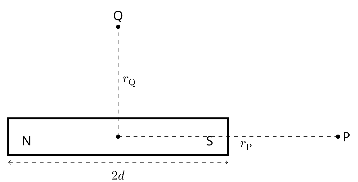
The magnitude of the magnetic field of a bar magnet in the axial direction at point P ( $B_{\mathrm{axial}}$ ) and at point $Q$ on its perpendicular bisector ( $B_{\mathrm{equatorial}}$ ) is given by the following formulae

B_{\mathrm{axial}} = \frac{\mu_0}{4\pi}\frac{2Mr_{\mathrm{P}}}{(r_{\mathrm{P}}^2 - d^2)^2} \qquad (1)

B_{\mathrm{equatorial}} = \frac{\mu_0}{4\pi}\frac{M}{(r_{\mathrm{Q}}^2 + d^2)^{3/2}} \qquad (2)

where $\mu_0$ is the permeability of free space ( $\mu_0/4\pi = 10^{-7}\mathrm{NA}^{-2}$ ), and $r_{\mathrm{P}}, r_{\mathrm{Q}}$ are the distances between the center of the magnet to the points where the field is measured. For the given problem, consider the magnet to be a point dipole ( $d \ll r_{\mathrm{P}}, r_{\mathrm{Q}}$ ).

Click on "EQ1-Magnetic Black Box" link in the exam portal for the experimental exam.

About the simulation on the screen:
You will see a canvas with a white background in the form of a grid on the screen. This grid canvas is a part of the vertical plane where the experiment is being carried out. There are four objects on the canvas:

a smartphone
a magnet in blue (S) and red (N) color
a dark shaded hollow pipe with uniform thickness
a calibrated scale, which can be activated by clicking the 'SHOW/HIDE SCALE' button.

Intergrid spacing on the grid canvas is 1 cm.

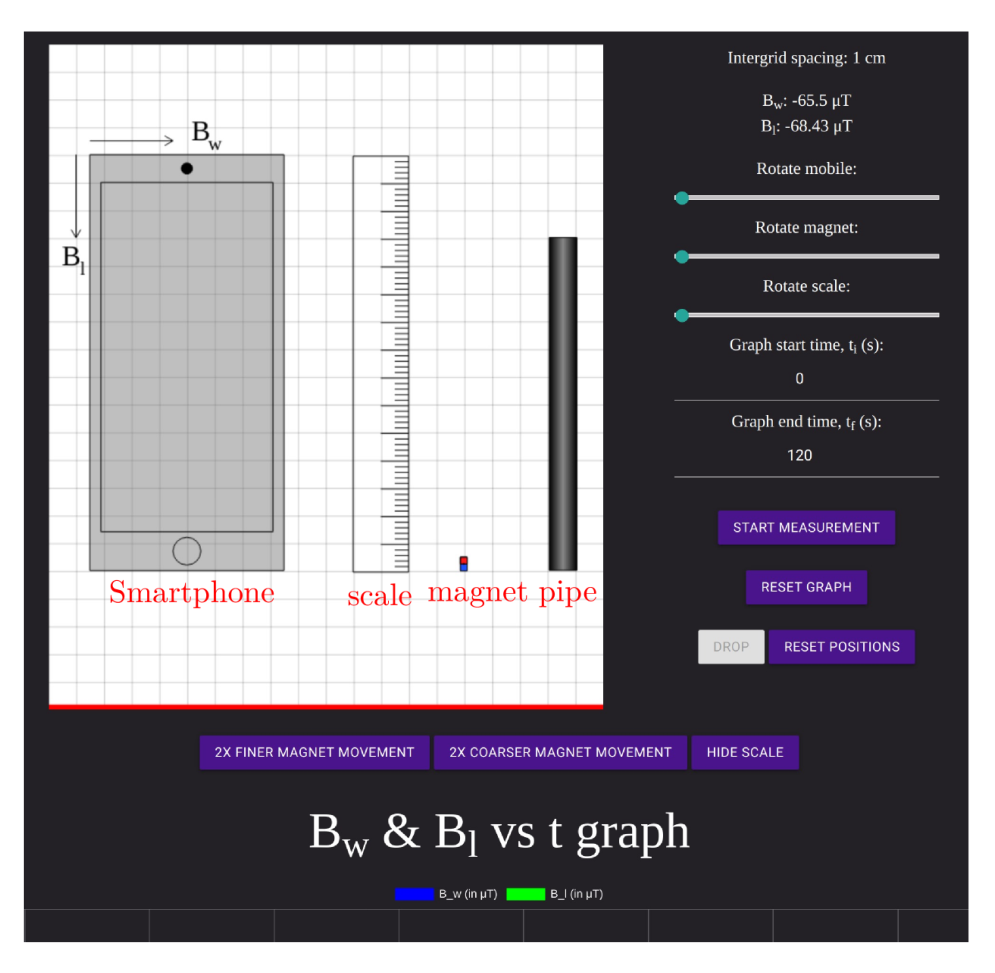
Screenshot of the simulation: a white grid canvas with a smartphone (arrows B_w to the right and B_l downwards, a black dot near its top), a scale, a small magnet and a dark pipe, labelled Smartphone, scale, magnet, pipe, and a red floor line. The dark right panel shows Intergrid spacing: 1 cm, readings B_w: -65.5 μT and B_l: -68.43 μT, sliders Rotate mobile, Rotate magnet, Rotate scale, fields Graph start time t_i (s): 0 and Graph end time t_f (s): 120, and buttons START MEASUREMENT, RESET GRAPH, DROP, RESET POSITIONS. Below: buttons 2X FINER MAGNET MOVEMENT, 2X COARSER MAGNET MOVEMENT, HIDE SCALE and the heading B_w & B_l vs t graph. — Figure 2: Screenshot of the simulation

The set up:
The objects can be moved by holding and dragging the mouse. Smartphone, scale, and magnet can also be rotated in the plane. The rotation control slider is available in the right panel. You can drag the slider to change the orientation. For a better control, after clicking on the slider, you can use arrow keys to rotate an object.
There is a magnetometer inside the phone which measures the magnetic field of the magnet in its vicinity. The exact location of the magnetometer in the phone is not given to you. Depending on the location of the magnetometer, the right panel displays the components $B_w$ and $B_l$ of the magnetic field of the magnet measured by the smartphone along its width and length, respectively, as shown in Fig 2. Component $B_w$ points to the right for the default position (portrait/vertical orientation) of the phone. Component $B_l$ points downwards along the length of the phone.

The measurement:
When you click on 'START MEASUREMENT' you can also see the graph of variation of $B_w$ and $B_l$ as a function of time. 'RESET GRAPH' will erase all the values recorded in this graph. When you move the cursor over the curve in the graph obtained, you can see the value of the data point. A portion of the graph can be zoomed in by inserting the time in the "Graph start time ( $t_i$ )" and the "Graph end time ( $t_f$ )" fields.

Smartphones may get damaged if they are exposed to high magnetic field. To prevent this, if the net magnetic field value measured by the smartphone exceeds 6500 $\mu$ T, the measurement will stop and you will see a warning on the right panel 'Maximum Magnetic field exceeded.' Measurement is restored as soon as the magnet is moved away from the phone at a sufficient distance.

Further features:
The magnet can be moved by keyboard arrow keys in up-down and left-right directions. For this, click anywhere on the canvas. A finer/coarser movement of the magnet can be achieved by clicking '2X FINER MAGNET MOVEMENT/2X COARSER MAGNET MOVEMENT'. With each clicking of these buttons, the movement will become two times finer/coarser. The buttons will grey-out when the maximum coarse/finer level is reached.

Gravity is in the downward direction, towards the bottom of the screen. The floor is indicated by a red line. Consider all the objects in the plane of the screen only. More information about the pipe is given before the part (B).

Consider the magnet to be held in a stationary position when you place it anywhere on the screen. Clicking on the "Drop" button will release the magnet and it will start descending. Note that the magnet can be dropped only after clicking the 'START MEASUREMENT' button. The 'RESET POSITION' button will bring back the magnet to the position from where it was dropped last. Objects can be moved outside the Canvas if needed.

In this experiment, consider the magnet to be a point dipole.
Note that there is no error estimation required in this question.

$^1$ Chandan Relekar (IISc, Bangalore), Siddhant Mukherjee (The University of Cambridge, UK), Siddharth Tiwary (IIT Powai, Mumbai), Charudutt Kadolkar (IIT Guwahati), Praveen Pathak (HBCSE-TIFR, Mumbai), were the principal authors of this problem. The contributions of the Academic Committee and the International Board are gratefully acknowledged.

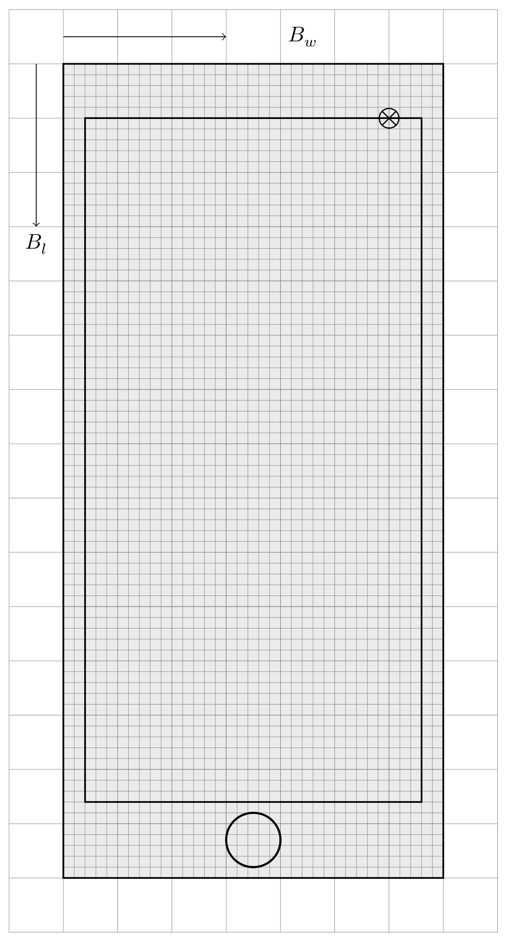
A.1 Obtain the location of the magnetometer on the phone. To help you answer this part in the answer sheet, a finer grid is made inside the schematic diagram of the phone. Intergrid spacing in the finer grid is 2 mm. Indicate the location of the magnetometer by drawing " $\otimes$ " in the smartphone at an appropriate place. [1 т.]

A.2 Plot a suitable linear graph and obtain the dipole moment of the magnet from the graph. Fill in the table for the recorded data of the method you have employed. [2,3 т.]

A hollow nonmagnetic vertically held pipe of finite uniform thickness is given on the screen. For the magnet to be dropped inside the pipe, the magnet should be aligned with the axis of the pipe properly. The "DROP" button will release the magnet in the vertical plane. The motion of the magnet inside the pipe cannot be viewed. Assume that when the magnet is dropped inside the pipe, it doesn't tilt or rotate as it descends. The pipe consists of three distinct sections: one section is made of wood (W), another section is made of aluminum (Al) having electrical conductivity $= 3.77 \times 10^7 \Omega^{-1}\mathrm{m}^{-1}$ , and the remaining section is made of copper (Cu) having electrical conductivity $= 5.96 \times 10^7 \Omega^{-1}\mathrm{m}^{-1}$ . These three different materials may/may not be in this order. If the magnet is dropped vertically (say along the downward $y$ -axis), the fall of the magnet is governed by

m\ddot{y} = mg - k\dot{y} \qquad (3)

where $m$ is the mass of the magnet, $g$ is the acceleration due to gravity ( $g = 9.8\mathrm{m/s^2}$ ), and $k$ is the damping constant due to the generation of the eddy current in the pipe. The damping constants for the wooden, aluminum, and the copper sections are zero, $k_{\mathrm{Al}}$ , and $k_{\mathrm{Cu}}$ , respectively. Drop the magnet inside the pipe following these steps:

Position the phone, the magnet and the pipe suitably.
Click the "Start Measurement" button.
click the "DROP" button.

The magnetometer can not measure very small magnetic field produced due to the eddy current in the pipe. As the magnet descends through the pipe, a graph of $B_w$ and $B_l$ as a function of time may be seen on the screen.

B.1 From the graph of the magnetic field vs time shown on the screen, find out the sequence of sections of different materials in the pipe. Indicate your answer by writing the number next to the material of the pipe considering them in order from top to bottom: 1 for the top section, 2 for the middle section, and 3 for the bottom section. [0,3 т.]

B.2 Determine the terminal velocity of the magnet in the Aluminium section of the pipe, plotting a suitable linear graph.
A canvas grid similar to the simulation screen is given in the answer sheet. Draw the schematic smartphone, pipe, and magnet to the exact locations and orientations you have used to obtain the data for this part. Use a box to indicate the Phone.
Fill tables with the relevant data set you are using for plotting the graph. Determine the length of the Aluminium section of the pipe. You may/may not use a graphical method for measuring the length of the aluminium section of the pipe. If you are using a graph/data set to determine the length, use the extra columns in the table to report the relevant data set. [2,6 т.]

B.3 Determine the terminal velocity of the magnet in the copper section of the pipe, plotting a suitable linear graph.
Determine the length of the copper section of the pipe. You may/may not use a graphical method for measuring the length of the copper section of pipe. If you are using a graph/data set to determine the length use the extra columns in the table to report the relevant data set. [2,2 т.]

B.4 Determine the length of the wooden section of the pipe. You may/may not use a graphical method for measuring the length of the wooden section of pipe. If you are using a graph/data set to determine the length use the extra columns in the table to report the relevant data set. [1,6 т.]

Отговори

Решение

EQ1: Official Solution

A.1 (1.0 pt)

Move the magnet along each of the axes and notice the change in the magnet field. For example, if the magnet is aligned along the length of the phone, and you are moving the magnet along the same direction (length of the phone), magnetic field will show the change in sign when the magnet crosses the Magnetometer.

Schematic of the smartphone on a coarse grid with a finer grid inside the phone body; arrows B_w (to the right, above the phone) and B_l (downwards, left of the phone); the home button circle at the bottom; the magnetometer marked ⊗ near the top right corner of the screen. — Figure. 1

[Figure. 1]

A.2 (2.3 pt)

The set up to find Dipole moment

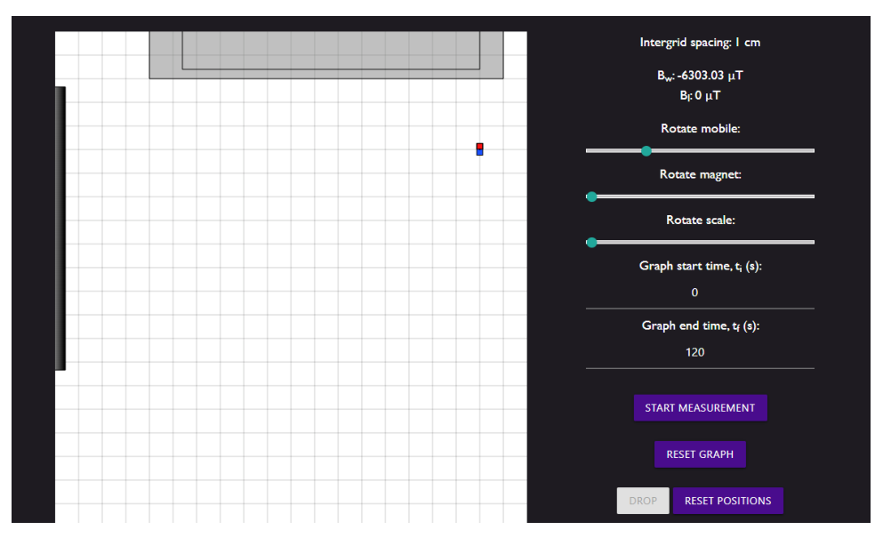
Screenshot of the set-up for finding the dipole moment: the phone rotated horizontally at the top of the canvas, the magnet to the right of it, the pipe at the left edge; the right panel shows B_w: -6303.03 μT, B_l: 0 μT, rotation sliders, graph start time 0, end time 120 and the buttons START MEASUREMENT, RESET GRAPH, DROP, RESET POSITIONS.

The magnetic field $B_w$ of a point dipole at the distance $x$ ( $x \gg d$ ) from the dipole's center can be approximated by

B_w = \frac{\mu_0}{2\pi}\frac{M}{x^3} \qquad (1)

Rearranging above equation, we get

B_w = \frac{\mu_0 M}{2\pi} \times \frac{1}{x^3} \qquad (2)

From equation (2), a plot of $B_w$ vs $\dfrac{1}{x^3}$ is a straight line passing through origin. Solving the slope will give dipole moment of the magnet.

A.2 (cont.)

Dipole moment of the Magnet:
Fill the appropriate quantities.

Sr.No	$x$ (cm)	$B_w(\mu\mathrm{T})$	$\frac{1}{x^3}(\mathrm{m}^{-3})$	$B_w$ (T)
1	5	3177.63	8000	0.00317763
2	6	1841.06	4629.63	0.00184106
3	7	1170.34	2915.45	0.00117034
4	8	783.69	1953.13	0.00078369
5	9	550.22	1371.74	0.00055022
6	10	403.42	1000	0.00040342
7	11	301.21	751.31	0.00030121
8	12	231.96	578.7	0.00023197
9	13	181.58	455.17	0.00018158
10	14	146.03	364.43	0.00014603
11	15	118.72	296.3	0.00011872
12	16	98.18	244.14	0.000099

From equation (2), a plot of $B_w$ vs $\dfrac{1}{x^3}$ is a straight line passing through the origin. The magnitude of the dipole moment can be calculated from the slope.

A.2 (cont.)

Graph of $B_w$ vs $\frac{1}{x^3}$

Graph of B (T), scale ·10^-3, from 0 to 3, versus 1/x^3 (m^-3) from 0 to 8,000: the data points lie on a straight line labelled 4.00 × 10^-7 X + 3 × 10^-6; legend: data.

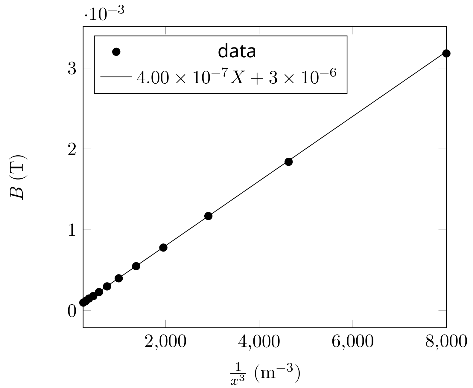
Slope of the graph: $4.00 \times 10^{-7}\ \mathrm{Nm}^2/\mathrm{A}$

Dipole moment of the magnet: 2.00 $\mathrm{Am}^2$

B.1 (0.3 pt)

Rotate the smartphone and align the magnet and the pipe along the width of the phone as shown below.

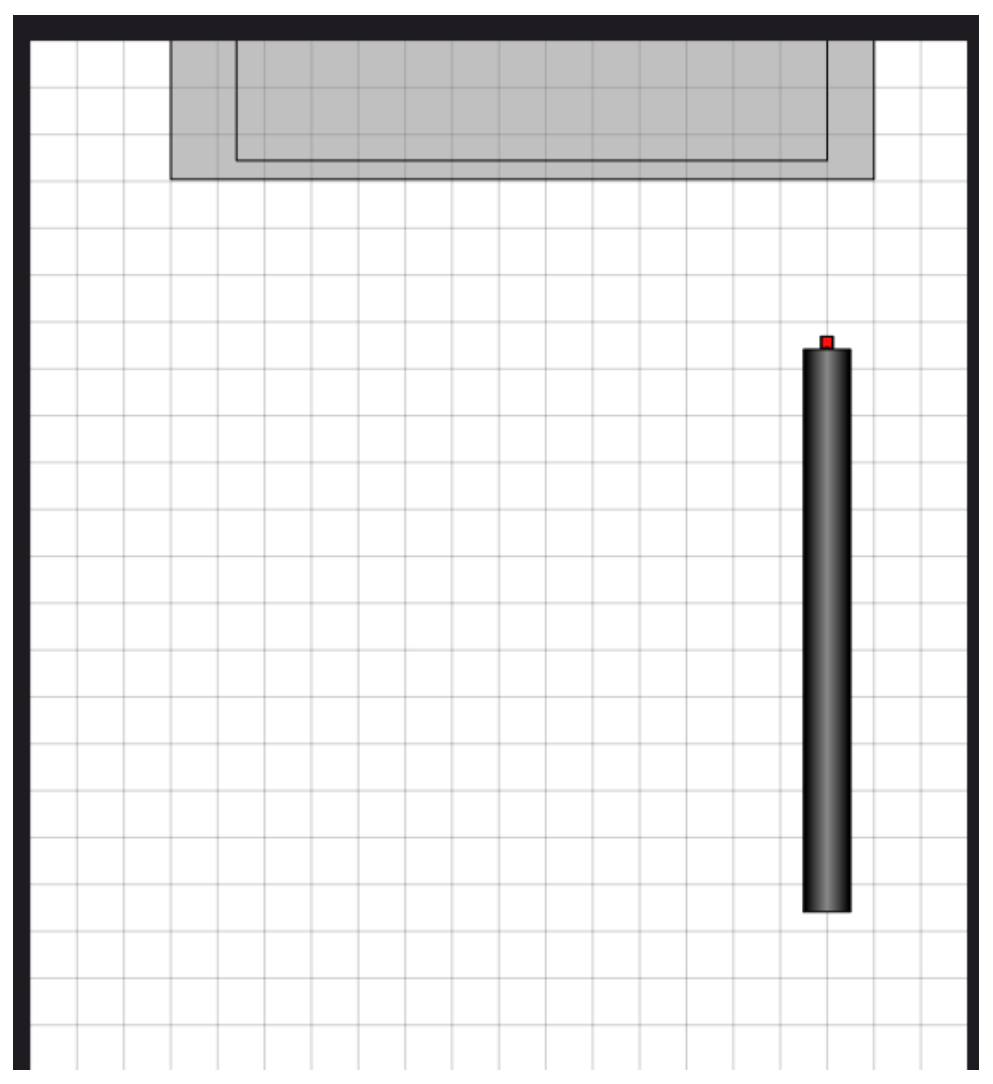
Canvas screenshot for part B: the phone rotated horizontally at the top of the canvas and the dark vertical pipe on the right with the small red-blue magnet at its top opening, aligned along the width of the phone.

Consider the case when the magnet is at rest at a distance $x_0$ from the magnetometer origin. The magnet is released along the axis of the pipe. It will start descending through the pipe. In the conducting sections of the pipe, after a brief period of accelerated motion, the magnet will attain a terminal velocity $v$ , due to the presence of eddy current damping. In this case, the magnetic field $B_w$ measured by the magnetometer changes with time $t$ as

B_w(t) = \frac{\mu_0}{2\pi}\frac{M}{(x_0 + vt)^3} \qquad (3)

Equation (3) is rearranged as

\left(\frac{\mu_0 M}{2\pi B_w(t)}\right)^{1/3} = vt + x_0 \qquad (4)

B.1 (cont.)

Obtained profile of magnetic field vs time clearly suggests three distinct phases (AB, BC, and CD) of the magnet's motion (see Fig. 4 below).

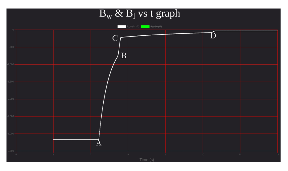
Screenshot of the B_w & B_l vs t graph on a dark background: B_w is flat at a large negative value until point A, rises steeply to B, rises again sharply to C, then increases very slowly to D and stays flat afterwards; horizontal axis Time (s). — Figure (4)

[Figure (4)]

We collect the data of ( $B_w$ vs $t$ ) for all three phases and plot them according to Eq. (4). For the acceleration phase of the pipe (wooden section), the graph will be non-linear and for the conducting pipe sections (Al and Cu) where the magnet moves with the terminal velocities, the graph will be linear. Duration of accelerated motion before attaining terminal velocity in the conducting sections of the pipe may be neglected.
It can be clearly seen from the graphs in the next sub parts that:

Section	Section number
Aluminium	1
Copper	3
wood	2

Since the copper has higher conductivity than aluminium, the terminal velocity in Cu section will be lower than Al section.

B.2 (2.6 pt)

Terminal velocity of Magnet in aluminium section:
Fill the appropriate quantities.

Sr.No	$B_w\ (\mu\mathrm{T})$	$t\ (\mathrm{s})$	$\left(\frac{\mu_0 M}{2\pi B_w(t)}\right)^{1/3}\ (\mathrm{m})$	$v\ (\mathrm{m/s})$
1	6462.28	0.534	0.0396	0
2	6462.28	0.536	0.0396	0.01
3	5954.24	0.558	0.0407	0.06
4	4850.05	0.606	0.0435	0.06
5	4002.02	0.654	0.0464	0.06
6	3651.48	0.678	0.0478	0.06
7	2817.43	0.75	0.0522	0.06
8	2397.97	0.798	0.055	0.06
9	1911.68	0.87	0.0594	0.06
10	1548.47	0.942	0.0637	0.06
11	1448.01	0.966	0.0651	0.06
12	1356.06	0.99	0.0666	0.06
13	1194.26	1.038	0.0694	0.06
14	1188.09	1.04	0.0696	0.14
15	1142.95	1.05	0.071

The velocity ( $v$ ) column is obtained using the forward difference $\dfrac{x_{n+1} - x_n}{t_{n+1} - t_n}$ .

From equation (4), a plot of $\left(\dfrac{\mu_0 M}{2\pi B_w(t)}\right)^{1/3}$ vs $t$ will be a straight line. The slope of the line will give terminal velocity .

B.2 (cont.)

Graph of $\left(\frac{\mu_0 M}{2\pi B_w(t)}\right)^{1/3}$ vs $t$

Graph of (μ0 M / 2π B_w(t))^(1/3) (m), scale ·10^-2, from 4 to 7, versus t (s) from about 0.55 to 1.04: the data points lie on the straight line 0.06X + 0.04; legend: data.

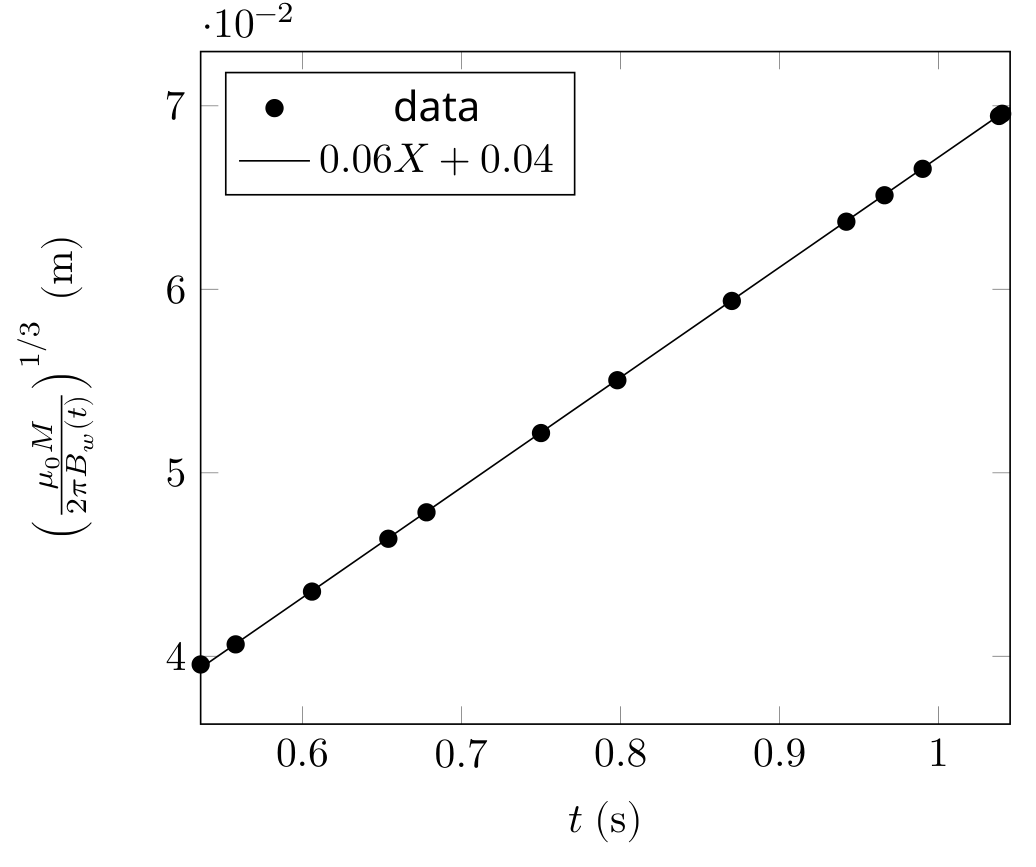
Slope of the graph: $6\ \mathrm{cm/s}$ .

Terminal velocity of the magnet in aluminium section: $6\ \mathrm{cm/s}$

Length of the aluminium section:

Slope of the graph: Not used — Intercept of the graph: Not used

Values in the fourth column in the above table actually represents the distance of the magnet from the magnetometer. We calculate the velocity (column 5) of the magnet using the forward difference method. Notice that the magnetic field starts to change at 0.536 s. Hence this is the point at which the magnet starts descending. It quickly achieves the terminal velocity of $6\ \mathrm{cm/s}$ . A change in velocity (or departure from the flat line in $v$ vs $t$ curve, if you plot) occurs at 1.040 s. This suggests that the magnet moved out of the aluminium section of the pipe at this time.

Length of the Al section $= (1.040 - 0.536) \times 6\ \mathrm{cm} = 3.024\ \mathrm{cm}$ .

B.3 (2.2 pt)

Terminal velocity of magnet in copper section:
Fill the appropriate quantities.

Sr.No	$B_w\ (\mu\mathrm{T})$	$t\ (\mathrm{s})$	$\left(\frac{\mu_0 M}{2\pi B_w(t)}\right)^{1/3}\ (\mathrm{m})$	$v\ (\mathrm{m/s})$
1	338.23	1.122	0.106	0.85
2	322.39	1.124	0.1075	0.87
3	271.32	1.244	0.1138	0.02
4	254.86	1.364	0.1162	0.02
5	239.70	1.484	0.1186	0.02
6	189.79	1.964	0.1282	0.02
7	169.97	2.204	0.1330	0.02
8	137.91	2.684	0.1426	0.02
9	131.17	2.804	0.1450	0.02
10	118.96	3.044	0.1498	0.02
11	108.22	3.284	0.1546	0.02
12	103.34	3.404	0.1570	0.02
13	98.52	3.53	0.1595	0.02
14	98.44	3.532	0.1596	0.02
15	98.37	3.534	0.1596	0.02
16	98.30	3.536	0.1597	0.05
17	98.22139	3.538	0.1597

The velocity ( $v$ ) column is obtained using the forward difference $\dfrac{x_{n+1} - x_n}{t_{n+1} - t_n}$ .

From equation (4), a plot of $\left(\dfrac{\mu_0 M}{2\pi B_w(t)}\right)^{1/3}$ vs $t$ will be a straight line. The slope of the line will give the terminal velocity.

B.3 (cont.)

Graph of $\left(\frac{\mu_0 M}{2\pi B_w(t)}\right)^{1/3}$ vs $t$

Graph of (μ0 M / 2π B_w(t))^(1/3) (m) from about 0.105 to 0.16 versus t (s) from about 1.1 to 3.5: the data points lie on the straight line 0.02X + 0.08893, except the first point which lies below it; legend: data.

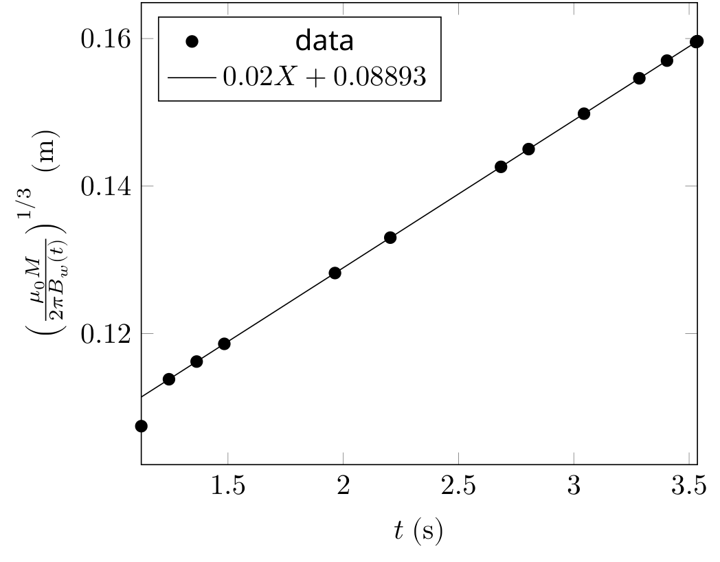
Slope of the graph: $2\ \mathrm{cm/s}$ .

Terminal velocity of magnet in copper section: $2\ \mathrm{cm/s}$

Length of copper section:

Slope of the graph: Not used — Intercept of the graph:Not used

Length of the copper section of the pipe can be calculated by $v_c t_c$ , where $v_c$ is the terminal velocity of the magnet in the copper section of the pipe and $t_c$ is the time spent by the magnet in the copper section of the pipe.
Data in the above table suggests that the magnet enters the copper section at $1.124\,\mathrm{s}$ , and it leaves the copper section of the pipe at $3.536\,\mathrm{s}$ where we see sudden velocity change.
Length of the copper section $= (3.536 - 1.124) \times 2\ \mathrm{cm} = 4.824\,\mathrm{cm}$ .

B.4 (1.6 pt)

Length of wooden section:
Fill the appropriate quantities.

Sr.No	$B_w\ (\mu\mathrm{T})$	$t\ (\mathrm{s})$	$\left(\frac{\mu_0 M}{2\pi B_w(t)}\right)^{1/3}\ (\mathrm{m})$	$v\ (\mathrm{m/s})$	$a\ (\mathrm{m/s^2})$
1	1194.26	1.038	0.0694	0.06	4
2	1188.09	1.04	0.070	0.14	5.66
3	1142.95	1.05	0.071	0.15	9.8
4	1056.94	1.06	0.072	0.25	9.8
5	941.55	1.07	0.075	0.34	9.8
6	811.40	1.08	0.079	0.44	9.8
7	679.75	1.09	0.084	0.54	9.8
8	556.44	1.1	0.090	0.64	9.8
9	447.31	1.11	0.096	0.74	9.8
10	354.74	1.12	0.104	0.83	9.8
11	338.23	1.122	0.106	0.85	-334.92
12	322.39	1.124	0.108	0.18	0.31
13	271.32	1.244	0.114

The velocity ( $v$ ) and acceleration ( $a$ ) columns are obtained using the forward difference $\dfrac{x_{n+1} - x_n}{t_{n+1} - t_n}$ and $\dfrac{v_{n+1} - v_n}{t_{n+1} - t_n}$ respectively.

B.4 (cont.)

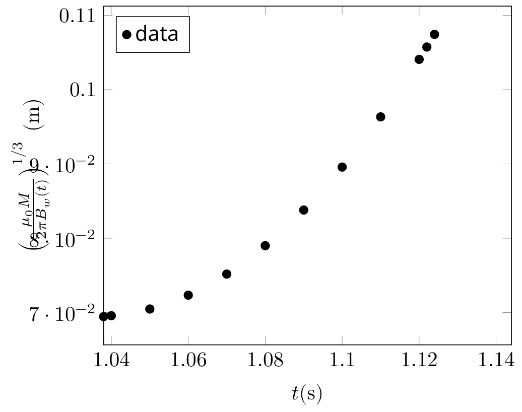
Graph of (μ0 M / 2π B_w(t))^(1/3) (m) from 7·10^-2 to 0.11 versus t(s) from 1.04 to 1.14: the data points rise along an upward-curving (non-linear) path from about 0.069 at 1.04 s to about 0.108 at 1.124 s; legend: data.

Wooden section is the middle section of the pipe. We have already established in Al section that the magnet exits the Al section at $1.040\ \mathrm{s}$ . We tabulate the data of velocity vs time for this section. Notice that the velocity of the magnet suddenly drops at $1.124\ \mathrm{s}$ . At this moment, the magnet enters in the copper section of the pipe and comes under the influence of damping due to the eddy current.
Length of the pipe can be calculated by $\left(v_{\mathrm{Al}} t_w + \frac{g t_w^2}{2}\right)$ , where $v_{\mathrm{Al}}$ is terminal velocity of magnet in the aluminium section of the pipe and $t_w$ is the time spent by the magnet in the wooden section of the pipe.
Total time spent by the magnet in the wooden pipe $(t_w) = (1.124 - 1.040)\ \mathrm{s} = 0.084\ \mathrm{s}$
Length of the wooden section of pipe $= 3.96\ \mathrm{cm}$

Оригинал в Архива: experiment-Q1-question.pdf · официални решения: experiment-Q1-solution.pdf