Съдържание

APhO 2022, Теория — Задача 2. A Mechanical Model for Phase Transitions

Оригинал на условието (PDF)Съобщи за грешка

Всички материали от APhO 2022

Theory — APhO INDIA 2022, 22nd Asian Physics Olympiad — Q2, Official (English)

Условие

A ring of radius $R$ has a bead of negligible size and mass $m$ threaded on it. The ring is set rotating about its vertical diameter with angular velocity $\omega$ as shown in Fig. 1. Alongside this, there is an opposing force on the bead, $F_f$ , which is proportional to the normal reaction $N$ , and is given by $F_f = fkN$ where $f$ is $1$ or $-1$ . You are advised to employ polar coordinates $\{r,\ \theta\}$ . As far as possible express your answers in terms of $\omega_c = \sqrt{g/R}$ where $g$ is the magnitude of the acceleration due to gravity.

In a phase transition the free energy, $V(\mathcal{M})$ [mechanical equivalent is potential energy] depends on the magnetization $\mathcal{M}$ as follows

V(\mathcal{M}) = a(T)\mathcal{M}^2 + b(T)\mathcal{M}^4

where $T \rightarrow$ temperature, $b(T) > 0$ and $a(T)$ changes sign with temperature. We attempt to understand the phenomenon of phase transition using the above mentioned model.

Note 1: For circular motion of radius $R$ , the velocity in polar coordinates is $\dot{\vec{r}} = R\dot{\theta}\hat{\theta}$ and the acceleration is $\ddot{\vec{r}} = -R\dot{\theta}^2\hat{r} + R\ddot{\theta}\hat{\theta}$ . Here $\hat{r}$ and $\hat{\theta}$ are unit vectors in the radial and the tangential directions respectively.

Note 2: The direction of the opposing force say $\vec{F}_f$ will be denoted by $f$ . Here $f$ = +1 if the bead is moving in the counter-clockwise direction (of increasing) $\theta$ and $f$ = -1 if the bead is moving in the clockwise direction $\theta$ , e.g. $f$ = $sgn(\dot{\theta})$ where $sgn$ is +1 or -1 depending on whether its argument is positive or negative.

Note 3: You may find the expansions

\begin{aligned} \sin(\theta) &= \theta - \theta^3/6 + .. \\ \cos(\theta) &= 1 - \theta^2/2 + \theta^4/24 + .. \\ (1+x)^n &= 1 + nx + n(n-1)x^2/2 + n(n-1)(n-2)x^3/6 + .. \end{aligned}

(where $\theta$ is in radians and $|x| \ll 1$ ) useful for some parts of the problem.

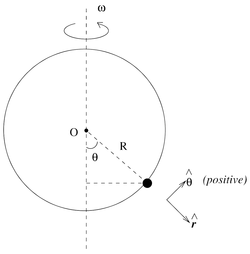
A circle (the ring) of centre O with a vertical dashed axis through O; a curved arrow at the top labelled ω shows rotation about the axis. A dashed radius R goes from O to the bead (black dot) at angle θ from the downward vertical; a dashed horizontal line joins the bead to the axis. Beside the bead, unit vectors θ̂ (positive) and r̂ are drawn. — Fig. 1: The bead on a rotating ring.

In what follows we shall understand the dynamics of the bead in the frame of the rotating ring and for angles in the range $-\pi/2 < \theta < \pi/2$ . The free body diagram of the bead is shown in Fig.2. Neglect all forces other than the ones shown in the free body diagram.

Lower half of the ring with a dashed vertical axis and rotation arrow ω; the bead at angle θ from the vertical. Forces on the bead: N along the radius towards the centre, mg vertically down, a dashed horizontal arrow mω²R sin θ outward, and the friction force F_f = fkN tangent to the ring. — Fig. 2: The free body diagram.

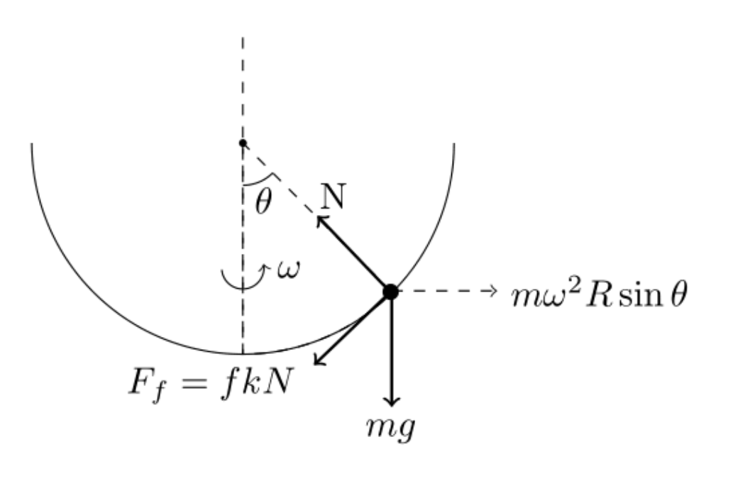
A.1 Write down the equations of motion for the radial $F_r$ and the tangential $F_\theta$ components of the force on the bead. Assume $\theta$ increasing in the counter-clockwise direction. [0,5 т.]

For the following parts B.1 to B.9 assume $k = 0$ .

B.1 State the relation between the equilibrium angle(s) $\theta_0$ in terms of $\{\ \omega,\ \omega_c\}$ . [1 т.]

B.2 Qualitatively sketch $\theta_0$ ( $y$ -axis) as a function of $\omega/\omega_c$ ( $x$ -axis). [0,5 т.]

B.3 Qualitatively sketch the magnitude of the normal reaction force on the bead as a function of $\omega/\omega_c$ at stable equilibrium. [0,5 т.]

B.4 We define the potential energy corresponding to the tangential force $F_\theta$ , namely

F_\theta = -\frac{1}{R}\frac{d}{d\theta}V(\theta)

with the zero of potential energy at $\theta = 0$ . If $V(\theta)$ is expressed as $P + Q\cos(\theta) + S\sin^2(\theta)$ , obtain $P, Q, S$ . [1 т.]

B.5 One can expand $V(\theta)$ for small $\theta$ and express it as $V(\theta) = a(\omega)\,\theta^2 + b(\omega)\,\theta^4$ . Obtain the coefficients $a(\omega)$ and $b(\omega)$ . [1 т.]

B.6 Make representative plots of $V(\theta)$ versus $\theta$ for values of $\omega/\omega_c$ just less than 1.0 (e.g. say 0.9) and $\omega/\omega_c$ large, say 5.0. Note that only qualitative sketches and no detailed calculations for the plots are required. [1 т.]

B.7 Landau theory of second order phase transitions can be used to demarcate simple magnetic systems into two phases. For temperatures $T$ greater than the critical temperature $T_c$ the system is paramagnetic. For $T < T_c$ the system is ferromagnetic and the magnetization $\mathcal{M}$ is given by

\mathcal{M}(T) = \mathcal{M}_0(1 - T/T_c)^{1/2} \quad T < T_c

Let us denote the exponent $1/2$ by $\beta$ . Compare this behaviour with the bead problem discussed above. What are the analogues of $\mathcal{M}$ , $T_c$ , $T/T_c$ in our case? What is the equivalent value of $\beta$ in our case? [1 т.]

B.8 Determine the angular frequency of oscillation $\Omega_0$ of the bead when it is disturbed from its “equilibrium” position $\theta_0$ . Note that for small oscillations

\Omega_0 = \frac{1}{R}\sqrt{\frac{V''(\theta_0)}{m}}

[1 т.]

B.9 Qualitatively sketch $\Omega_0$ as a function of $\omega$ . [1 т.]

For the following parts C.1 to C.2 $k \neq 0$ .

C.1 Take $f$ = 1 and express $k = \tan\alpha$ . We may express the condition for the equilibrium angle(s) $\theta_0$ as

\left(\frac{\omega}{\omega_c}\right)^2 = \frac{\tan(x)}{\sin(y)}

Obtain $x$ and $y$ . [1 т.]

C.2 It is given that $f$ =1 and $k = 0.05$ . Obtain the equilibrium angles $\theta_0$ , if any, for the following cases:

$\omega/\omega_c$ = 0.50
$\omega/\omega_c$ = 0.70 [0,5 т.]

¹Sitikantha Das (IIT Kharagpur) and Pramendra Ranjan Singh (Principal, Narayan College, J.P. University) were the principal authors of this problem. The contributions of the Academic Committee, Academic Development Group, and the International Board are gratefully acknowledged.

Отговори

Решение

General Grading Guidelines

When student’s solutions are correct and s/he also show how solutions were obtained, the stduent gets full credit. The scheme oulined below is helpful if the student’s answers are partially correct. Attention will be paid to the detailed solution so, if the final answer is correct but it is obtained by incorrect method(s) then no credit will be given. Alternative solutions may exist and will be given due credit.

Partial or full outcomes obtained for later sections in the problem which are incorrect solely because of errors being carried forward from previous sections, but are otherwise reasonable, will not be further penalized. For example a dimensioanlly wrong answer when carried forward will not get any credit in the subsequent sections. A numerically wrong evaluation when carried forward will get credit in subsequent sections unless the numerical answer is patently wrong (e.g. the value of g is 981 m/sec $^2$ ! )

Incorrect or no labeling of an axis is penalized by -0.1 points

The numerical answer (i) must be correct to +/- 10% AND (ii) must respect significant figures.

It maybe noted that NO micro-marking scheme takes care of all contingencies. A certain amount of discretion rests with and a certain level of judgement is invested in the academic committee.

A.1 (0.5 pt)
Equations of motion

The radial component $F_r$ yields:

mR\dot{\theta}^2 = N - mg\cos(\theta) - mR\sin^2(\theta)\omega^2 \qquad (1)

[0.2]

The tangential component $F_\theta$

mR\ddot{\theta} = mR\sin(\theta)\cos(\theta)\omega^2 - mg\sin(\theta) - \mathrm{sgn}\left(\dot{\theta}\right)kN \qquad (2)

mR\ddot{\theta} = mR\sin(\theta)\cos(\theta)\omega^2 - mg\sin(\theta) - fkN \quad (f = 1) \qquad (3)

[0.3]

No points if equations not written using radial and tangential components.

B.1 (1.0 pt)
Equilibrium angle(s)

We set $k = 0$ in the equation for the tangential component of the force. Thus

mR\ddot{\theta} = mR\sin(\theta)\cos(\theta)\omega^2 - mg\sin(\theta) \qquad (4)

For equilibrium we set $\ddot{\theta}_0$ = 0 in the above equation. Then $\theta_0$ = 0 is an equilibrium angle for all values of $\omega$

[0.4]

The other values are given by

\cos\theta_0 = \frac{g}{\omega^2 R} = \frac{\omega_c^2}{\omega^2} \qquad (5)

[0.3]

\theta_0 = \pm\left|\cos^{-1}\frac{\omega_c^2}{\omega^2}\right| \qquad (6)

[0.1]

with values of $\theta_0$ between - $\pi/2$ to $\pi/2$ . The $\pm$ indicates that there are two equivalent positions. () The bead could rise on either side of the axis shown in the figure depicted in the problem. Note that for $\omega < \omega_c$ , Eq. (5) implies $\cos\theta_0 > 1$ . This is clearly unphysical. A little reflection will convince us that $\theta_0 = 0$ for $\omega < \omega_c$ .

[0.2]

B.2 (0.5 pt)
Sketch of $\theta_0$ .

Sketch of θ0 (vertical axis, 0 marked) against ω/ωc (horizontal axis, 1 marked): θ0 = 0 for ω/ωc < 1; at ω/ωc = 1 (dashed vertical line) it splits into two symmetric red branches rising and falling steeply and levelling off towards constant positive and negative values.

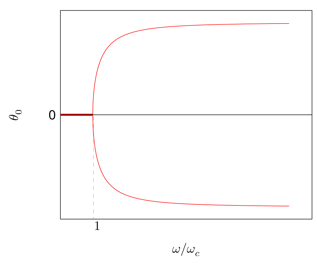
[shape correct: 0.2]
[only if both branches: 0.3]

B.3 (0.5 pt)
Sketch of the magnitude of the normal reaction

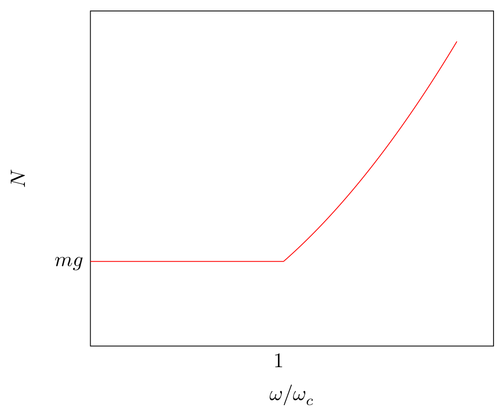
Sketch of N (vertical axis, mg marked) against ω/ωc (horizontal axis, 1 marked): N = mg constant up to ω/ωc = 1, then increasing (as mω²R) beyond it.

[ $\omega < \omega_c$ : 0.2]
[ $\omega > \omega_c$ : 0.3]

If the shape of the plot is wrong, in that case, the following would be used. If in the detailed work, it is shown that $N = mg$ for $\omega < \omega_c$ , 0.1 points would be provided. If it is shown that $N = m\omega^2 R$ for $\omega \geq \omega_c$ , 0.1 points would be provided.

B.4 (1.0 pt)
The potential $V(\theta)$

Solution 1: Using direct integration
Given that

F_\theta = -\frac{1}{R}\frac{dV(\theta)}{d\theta} \qquad (7)

and taking $V(\theta = 0) = 0$ , we obtain on integrating Eq. (4) that

-R\int_0^\theta F_\theta d\theta = \int_0^V dV = V - 0

[0.3]

the left hand side is

\begin{aligned} -R\int_0^\theta F_\theta d\theta &= \frac{-m\omega^2R^2}{2}\int_0^\theta \sin(2\theta) + mgR\int_0^\theta \sin(\theta)d\theta \\ &= \frac{m\omega^2R^2(\cos(2\theta) - 1)}{4} - mgR(\cos(\theta) - 1) \qquad (8) \end{aligned}

[0.4]

Noting that $cos(2(\theta) - 1) = -2\sin^2(\theta)$ and $\omega_c^2 = g/R$ we obtain

V(\theta) = mgR\left[(1 - \cos\theta) - \frac{\omega^2}{2\omega_c^2}\sin^2\theta\right] \qquad (9)

[0.3]

We can also verify the above equation by substitution into Eq. (7)
$P = mgR$
$Q = -mgR$
$S = -\dfrac{\omega^2 mgR}{2\omega_c^2}$

Solution 2: Differentiating $V = P + Q\cos(\theta) + S\sin^2(\theta)$
$F_\theta = mR\sin\theta\cos\theta\omega^2 - mg\sin\theta = -\dfrac{1}{R}\dfrac{dV(\theta)}{d\theta} = \dfrac{Q}{R}\sin(\theta) - 2\dfrac{S}{R}\sin\theta\cos\theta$

[0.3]

Comparing, we get,
$Q = -mgR$
$S = -\dfrac{\omega^2 mgR}{2\omega_c^2}$

[0.2,0.2]

Also, as $V(0) = 0$ , we have $P + Q = 0$ . Hence, $P = mgR$

[0.3]

B.5 (1.0 pt)
The coefficients

We use the expansions for the trigonometric functions $\sin(\theta)$ and $\cos(\theta)$ in Eq. (10). We shall keep terms upto and including order $\theta^4$ . Thus

\begin{aligned} V(\theta) &\approx mgR\left[1 - 1 + \theta^2/2 - \theta^4/24 - \frac{\omega^2}{2\omega_c^2}(\theta - \theta^3/6)^2\right] \\ &\approx \frac{mgR}{2}\left[1 - \frac{\omega^2}{\omega_c^2}\right]\theta^2 + \frac{mgR}{6}\left[\frac{\omega^2}{\omega_c^2} - \frac{1}{4}\right]\theta^4 \end{aligned}

Thus

a(\omega) = \frac{mgR}{2}(1 - \frac{\omega^2}{\omega_c^2})

[0.5]

b(\omega) = \frac{mgR}{6}(\frac{\omega^2}{\omega_c^2} - \frac{1}{4})

[0.5]

Note: no penalty if the 1/4 term is missed.
One observes that if one incorrectly expands $\sin\theta \approx \theta$ , in that case, only $a(\omega)$ will turn out to be correct.

B.6 (1.0 pt)
Representative plots of the potential

Solution 1: Plotting for $\theta \in [-\pi/2, \pi/2]$

V(θ) against θ for θ from −π/2 to π/2 (ticks −π/2, 0, π/2; 0 level dashed). Red curve (ω < ωc): single parabola-like well with minimum 0 at θ = 0. Blue curve (ω > ωc): maximum 0 at θ = 0 and two minima labelled −θ0 and θ0. Legend: ω < ωc, ω > ωc.

[ $\omega < \omega_c$ : 0.5]
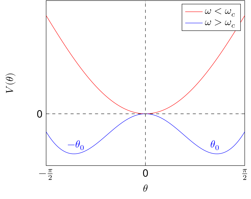
[ $\omega > \omega_c$ : 0.5]

Solution 2: Plotting for $\theta \in [-\pi, \pi]$

V(θ) against θ for θ from −π to π (ticks −π, 0, π; 0 level dashed). Red curve (ω < ωc): single well with minimum at θ = 0, rising to a maximum at ±π. Blue curve (ω > ωc): local maximum 0 at θ = 0, two minima labelled −θ0 and θ0, rising to the same maxima at ±π. Legend: ω < ωc, ω > ωc.

[ $\omega < \omega_c$ : 0.5]
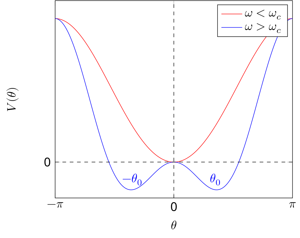
[ $\omega > \omega_c$ : 0.5]

B.7 (1.0 pt)
Bead analogues
Solution 1:
For $\omega \rightarrow \omega_c^+,\ \theta_0$ is close to zero. Hence on expanding the cosine term in Eq. (5),

\begin{aligned} 1 - \frac{\theta_0^2}{2} &= \frac{\omega_c^2}{\omega^2} \\ \theta_0 &= \pm\sqrt{2}\left[1 - \frac{\omega_c^2}{\omega^2}\right]^{1/2} \qquad (10) \end{aligned}

Also note from Eq. (5) that as $\omega \rightarrow \infty$ , $\theta_0 \rightarrow \pm\pi/2$ . This plot also has an analogue in phase transition. The magnetization $\mathcal{M}$ goes to zero as $T$ goes to $T_c$ in a similar fashion. Thus the role of $\mathcal{M}$ is played by $\theta_0$ and temperature is inversely related to $\omega$ . Increasing temperature is equivalent to decreasing $\omega$ . Summarizing,

\mathcal{M} \longrightarrow \theta

[0.4]

\begin{aligned} T_c &\longrightarrow 1/\omega_c^2 \\ T/T_c &\longrightarrow \omega_c^2/\omega^2 \end{aligned}

[0.4]

Equivalent value of $\beta$ for bead is = 1/2.

[0.2]

Solution 2:
For $\omega > \omega_c,\ \cos\theta_0 = \omega_c^2/\omega^2$ . Hence on writing $\sin^2\theta_0 = 1 - \cos^2\theta_0$ and substituting the value of $\cos\theta_0$ , one gets $\sin\theta_0 = (1 - \frac{\omega_c^4}{\omega^4})^{1/2}$ . This plot also has an analogue in phase transition. The magnetization $\mathcal{M}$ goes to zero as $T$ goes to $T_c$ in a similar fashion. Thus the role of $\mathcal{M}$ is played by $\sin\theta_0$ (or equivalently $\theta_0$ in the small angle limit) and temperature is inversely related to $\omega^4$ . Increasing temperature is equivalent to decreasing $\omega$ . Summarizing,

\mathcal{M} \longrightarrow \sin\theta

[0.4]

\begin{aligned} T_c &\longrightarrow 1/\omega_c^4 \\ T/T_c &\longrightarrow \omega_c^4/\omega^4 \end{aligned}

[0.4]

Equivalent value of $\beta$ for bead is = 1/2.

[0.2]

[Note: The critical exponent is $1/2$ in our case and also in Landau theory. However experimentally and in more elaborate theories the exponent of vanishing magnetization is $1/3$ ].

B.8 (1.0 pt)
Oscillation frequency

The frequency of oscillation $\Omega_0$ of the bead about the "equilibrium" position $\theta_0$ is

\Omega_0 = \frac{1}{R}\sqrt{\frac{V''(\theta)}{m}}

We take the second order derivative of the potential as given in Eq. (10)

V''(\theta) = mgR\cos\theta\left[1 - \frac{\omega^2}{\omega_c^2}\cos\theta\right] + mgR\,\frac{\omega^2}{\omega_c^2}\,\sin^2\theta \qquad (11)

For $\theta = \theta_0 = \pm\cos^{-1}(\omega_c^2/\omega^2)$

V''(\theta_0) = mgR\,\frac{\omega^2}{\omega_c^2}\left(1 - \frac{\omega_c^4}{\omega^4}\right) > 0 \qquad \text{if } \omega > \omega_c \qquad (12)

For $\omega < \omega_c$ , $\theta_0 = 0$ , and we obtain from Eq. (12) that

\Omega_0 = (\omega_c^2 - \omega^2)^{1/2} \qquad (13)

[0.5]

Similarly for $\omega > \omega_c$ , using Eq. (13) we obtain

\Omega_0 = \omega\left(1 - \frac{\omega_c^4}{\omega^4}\right)^{1/2} \qquad (14)

[0.5]

No credit will be provided is small angle approximation of $V(\theta)$ is used.

B.9 (1.0 pt)
Sketch of $\Omega_0$

Sketch of Ω0 against ω: red curve (ω < ωc) falls from Ω0 = ωc at ω = 0 to zero at ω = ωc; blue curve (ω > ωc) rises from zero at ω = ωc and approaches the dashed line Ω0 = ω from below. Legend: ω < ωc, ω > ωc.

[ $\omega < \omega_c$ : 0.5]
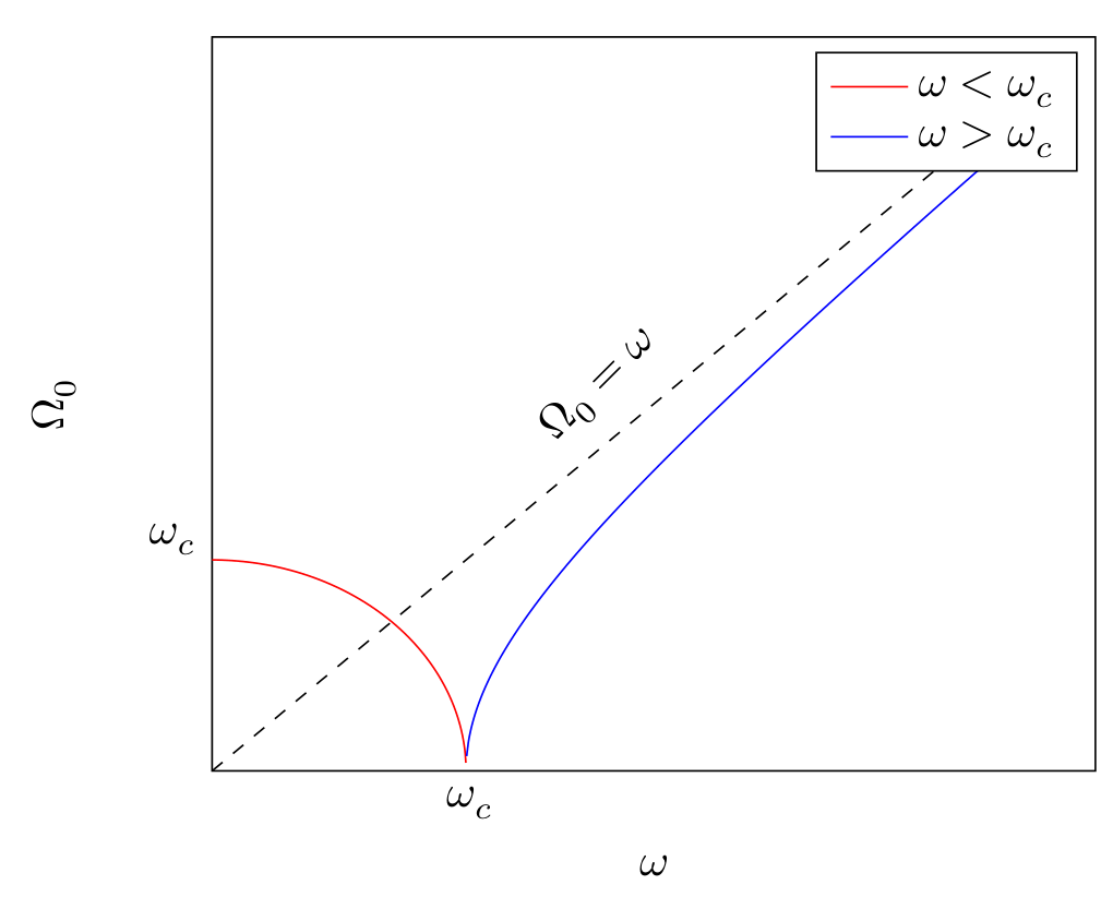
[ $\omega > \omega_c$ : 0.5]

In the case of wrong expression of $\Omega_0$ derived in the previous part, marks would be awarded based on the plot of expression obtained, and physicality of the plots.

C.1 (1.0 pt)
Condition for equilibrium angles

We substitute the expression for the normal reaction (Eq.(1)) in the angular part (Eq.(3)) to obtain

mR\ddot{\theta} = mR\sin(\theta)\cos(\theta)\omega^2 - mg\sin(\theta) - fk(mg\cos(\theta) + mR\sin^2(\theta)\omega^2 + mR\dot{\theta}^2)

Noting that $\omega_c^2$ = $g/R$ and rearranging terms we have

\ddot{\theta} = \omega_c^2\left[(\sin(\theta))\,(\cos(\theta) - fk\sin(\theta))\left(\frac{\omega}{\omega_c}\right)^2 - \sin(\theta) - fk\cos(\theta) - fk\left(\frac{\dot{\theta}}{\omega_c}\right)^2\right]

[0.2]

At equilibrium, $\dot{\theta} = 0,\ \ddot{\theta} = 0$ and $f = \mathrm{sgn}\left(\dot{\theta}\right) = \pm 1$ depending on how this equilibrium was attained, iė., depending on the value of $\dot{\theta}$ just before equilibrium was attained. Thus we obtain the expression for the equilibrium angle $\theta_0$ ,

\boxed{\sin(\theta_0)\,(\cos(\theta_0) - fk\sin(\theta_0))\left(\frac{\omega}{\omega_c}\right)^2 = \sin(\theta_0) + fk\cos(\theta_0) \ \text{with}\ \theta_0 \in (-\pi/2, \pi/2)}

[0.4]

For $f$ = 1 and $k = \tan(\alpha)$ we may express the above as

\begin{aligned} \left(\frac{\omega}{\omega_c}\right)^2 &= \frac{\sin(\theta_0) + \tan(\alpha)cos(\theta_0)}{\sin(\theta_0)(\cos(\theta_0) - \tan(\alpha)\sin(\theta_0))} \\ &= \frac{\tan(\theta_0 + \alpha)}{\sin(\theta_0)} \qquad (15) \end{aligned}

[0.4]

In case of algebraic error leading to $x = \theta_0 - \alpha$ , only 0.1 points would be deducted.

C.2 (0.5 pt)
Representative values for $\theta_0$
We are given the expansions for the trigonometric functions in the problem. We notice that the coefficient of the opposing force $k$ is small (=0.05). Thus $k$ = $\alpha$ . We then have

\sin(\theta_0) \approx \theta_0

\tan(\theta_0 + \alpha) \approx \theta_0 + \alpha

[0.2]

Thus

\left(\frac{\omega}{\omega_c}\right)^2 \approx 1 + \frac{k}{\theta_0}

Simple calculations yield (a) $\theta_0$ = -0.07 radians (b) $\theta_0$ = -0.1 radians

[0.3]

The plot will no longer be symmetric.

Оригинал в Архива: theory-Q2-question.pdf · официални решения: theory-Q2-solution.pdf