APhO 2023, experiment — Задача 1. Hertzian Contact Stress [10 points]

Experiment — APhO XXIII Mongolia 2023 — Q1, English (Official) · 10 т.

Условие

Please read the general instructions before you start this problem.

Introduction

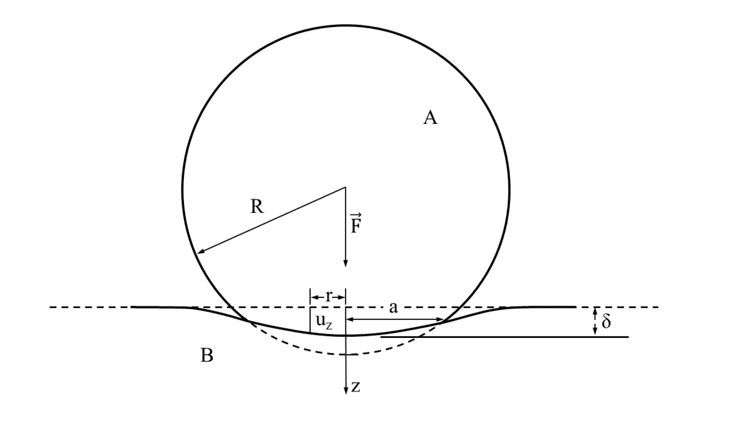
The Hertzian contact theory is a classical theory of contact mechanics and is a very useful tool for engineers and researchers. Even though the derivation of the theory is relatively difficult, the final solution is a set of simple analytical equations relating the properties of the system to the developed stress. Hertz contact theory is derived from the analytical solution of elasticity theory equations under the so called half-space approximation:

1. One of the surfaces is a half-space (one of two regions formed when a plane divides 3D Euclidean space) of infinite extend (Figure 1).
2. Pressure profile is parabolic (Equation 2)
3. This infinite half-space model can be used for two spherical balls with the same or different sizes.

If there are only vertical forces acting on the surface, the elastic deflection of the surface under applied pressure is given by the following relation:

$u_z(x,y) = \frac{2\pi}{E'} \iint \frac{p(x',y')}{\sqrt{(x-x')^2+(y-y')^2}}\,dx'\,dy' \qquad (1)$

Here $u_z$ is the elastic deflection, $\frac{1}{E'} = \frac{(1-v_1^2)}{E_1} + \frac{(1-v_2^2)}{E_2}$ is the reduced elastic modulus, $v_1, E_1, v_2, E_2$ are respectively the Poisson's ratio and Young's modulus (these values are constant for given balls and will be provided for calculations in task E.1) of the spheres, $p(x,y)$ is the contact pressure. If the pressure profile is arbitrary, this equation does not lead to the analytical solution. However, the Hertz solution is obtained under the assumption of a parabolic pressure distribution, which is a very good approximation for spherical, elliptical or cylindrical bodies in contact:

$p(r) = p_0\left(1 - \frac{r^2}{a^2}\right)^{1/2} \qquad (2)$

where $r$ is the distance to the arbitrary point on the surface and $a$ is a parameter known as the Hertz contact radius. Parameter $p_0$ is also called the maximum Hertz pressure. Substituting this into the Equation (1) for deflection leads to the following expression for the Hertzian pressure:

$u_z = \frac{\pi p_0}{4E' a}(2a^2 - r^2),\ r \leq a \qquad (3)$

This experimental problem has two parts: large angle pendulum and two balls collisions.

General Safety Precautions:

1. Be sure to switch off the equipment before plug in/out its power cord. Damage may occur.
2. Do not change the oscilloscope settings unless instructed in the problem.
3. Be careful not to spill the drinking water onto nearby electronics and electrical power sockets.
4. Do not disassemble the first experimental setup, unless you have finished the experiment. You would not be able to reassemble again.

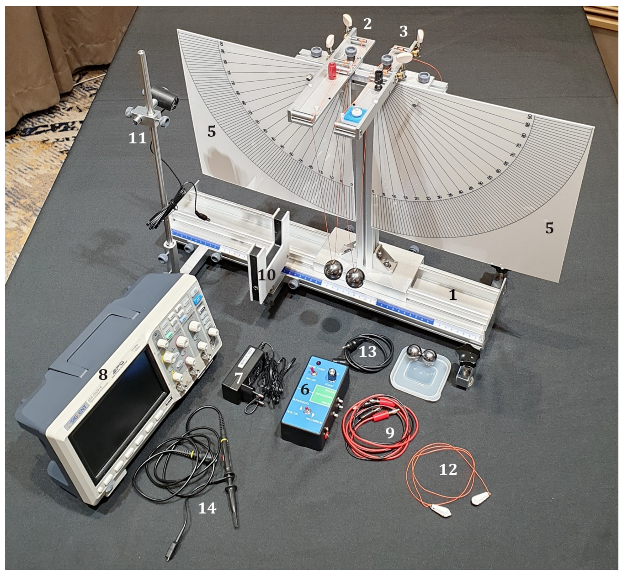
Apparatus

1. Base flatform of the setup. (Base will be used for both experiments)
2. Pendulum 1 with hanger unit (big ball is hung already).
3. Pendulum 2 with hanger unit (big ball is hung already).
4. Two small sized balls.
5. Angle measuring screens for Left and Right sides.
6. Electric junction box.
7. Power adaptor.
8. Oscilloscope with measuring probe 14.
9. Connecting wires for ball contact measurement.
10. Photogate for pendulum with connecting cable (13).
11. Electromagnetic ball holder with adjusting stand.
12. Wire with two plumb bobs.

Part A: Large angle pendulum [1.4 points]

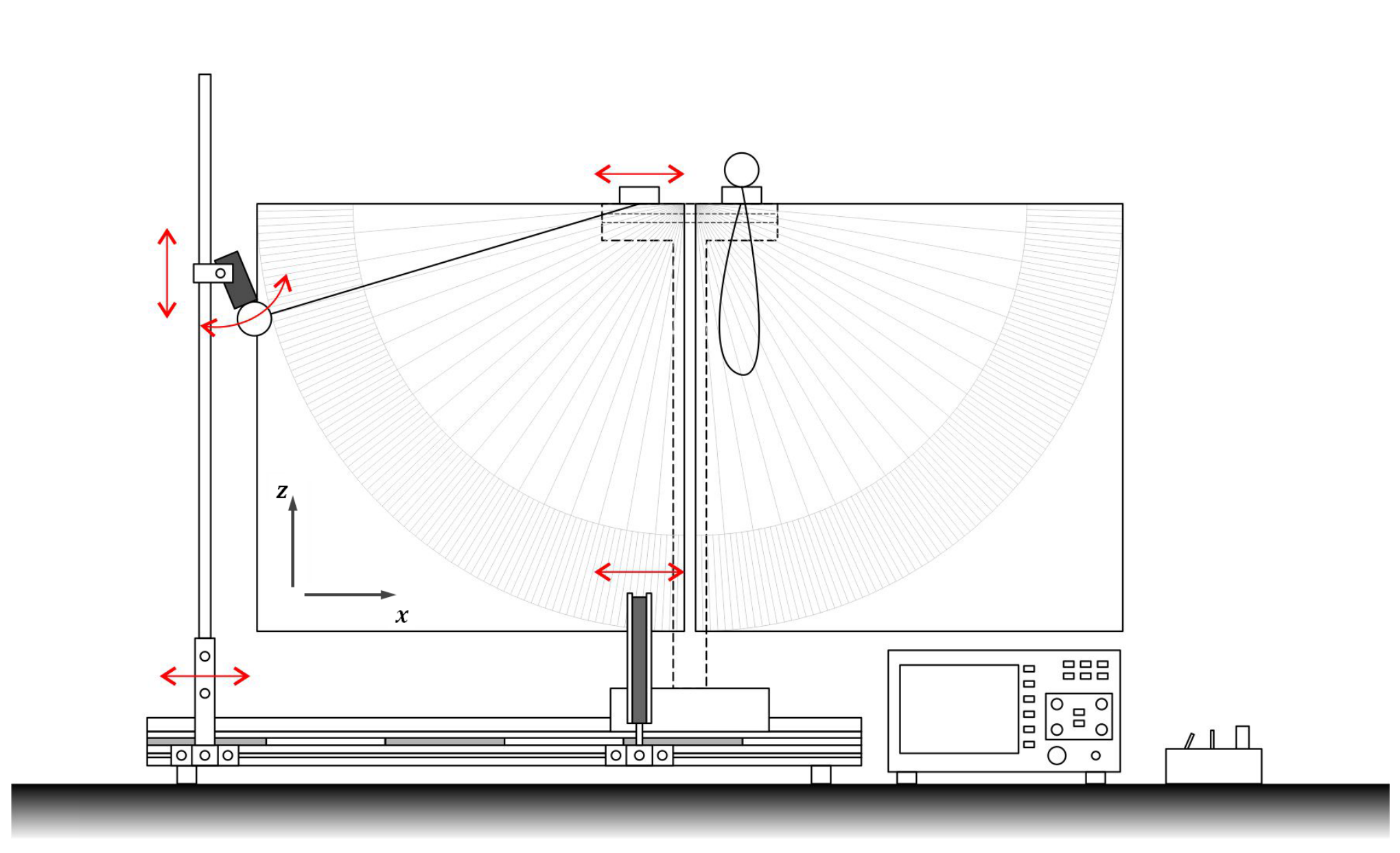
In this part, you are required to determine the maximum speed and angular amplitude relation of the single ball pendulum starting from large angle to small angle, for as wide a range of angles as possible. To use the pendulum, you should understand the ball position adjusting techniques. There are two string tuning knobs on each pendulum hanger. They are used for adjusting ball positions up/down for $z$ direction and forward/backward for $y$ direction. To adjust ball positions left/right for $x$ direction the pendulum hanger unit should be used (Figure 3).

For this task you are required to use only one of the pendulums. Therefore, please put one of the already fixed balls on the head of the screw for tightening pendulum hanger. Please pay attention to the pendulum wires to be not disturbing the movement of your working pendulum.

Part B: Period of the oscillation [1.9 points]

The period of the pendulum depending on the angular amplitude is given by the following series.

$T = T_0\left(1 + \alpha \cdot \sin^2\frac{\varphi_0}{2} + \beta \cdot \sin^4\frac{\varphi_0}{2} + \cdots\right) \qquad (4)$

Here $T_0$ is the pendulum period when amplitude is small, $\alpha$ and $\beta$ are constant coefficients, and $\varphi_0$ is the angular amplitude.

Part C: Behaviors of the collisions [0.7 points]

The initial positions and the conditions of the balls will strongly affect first collision and further collisions processes: position of collisions, contact time and contact positions on the balls. To execute this task please pay attention to the ball position adjusting techniques.

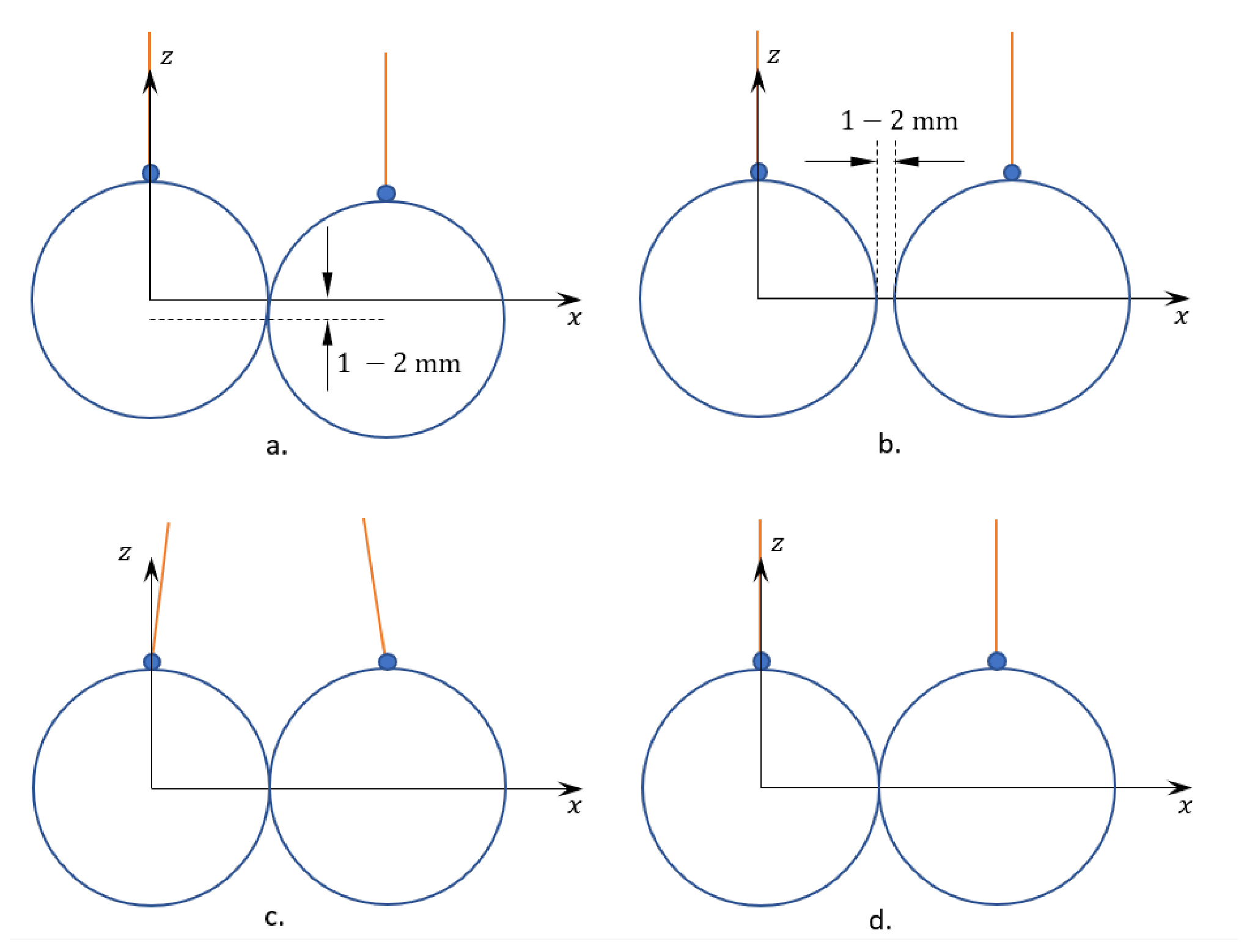
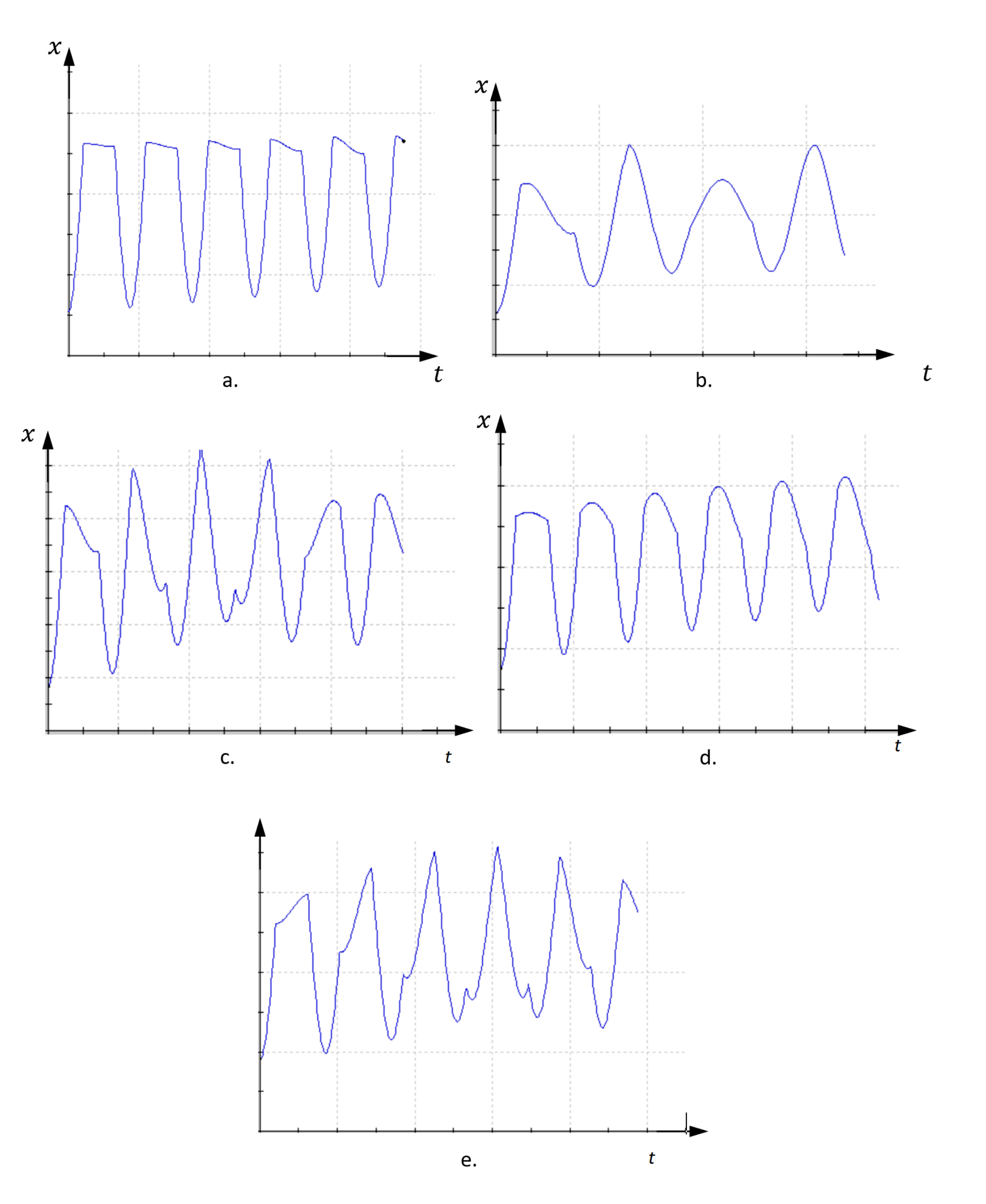
In this part you will observe the influence of the contact position on the behavior of the collisions of identically sized balls. Observe the behavior of the collisions for each of the scenarios described in sections C.1-C.4 (matching the appropriate description in Figure 4) and for each task match between the setup and a time dependence graph from Figure 5.

C.1 When two balls are hung and stable at the equilibrium position, we assume that the center of the first ball as the origin of the coordinate system. Then the positions can be described as: the displacement between two ball centers in $x$ direction $d_x = 2R$, displacement in $y$ direction $d_y = 0$, displacement in $z$ direction $d_z \approx 1$ to $2\ \mathrm{mm}$and the hanging wires are almost parallel (Figure 4.a). When ball 2 is in equilibrium position, ball 1 is released from angle from $25^\circ$ to $30^\circ$ without initial speed. Observe by eyes the influence of the contact position on the collision behavior of identically sized balls.

C.2 $d_x - 2R \approx 1\ \mathrm{mm}$, $d_y = 0$, $d_z = 0$ and two wires are parallel. That means the ball hanger units should be moved away by $1\ \mathrm{mm}$ distance (Figure 4.b). When ball 2 is in equilibrium position, ball 1 is released from an angle between $25^\circ$ to $30^\circ$ without initial speed. Observe by eyes the influence of the contact position on the collision behavior of identically sized balls.

C.3 The two balls are in contact, $d_x \approx 2R$, $d_y = 0$, $d_z = 0$ and the ball hanger units touch each other. In this case wires are not parallel (Figure 4.c). When ball 2 is in equilibrium position, ball 1 is released from an angle between $25^\circ$ to $30^\circ$ without initial speed. Observe by eyes the influence of the contact position on the collision behavior of identically sized balls.

C.4 The two balls are in contact, $d_x \approx 2R$, $d_y = 0$, $d_z = 0$ and the ball hanger units are separate, the ball wires are parallel (Figure 4.d). When ball 2 is in equilibrium position, ball 1 is released from an angle between $25^\circ$ to $30^\circ$ without initial speed. Observe by eyes the influence of the contact position on the collision behavior of identically sized balls.

Part D: Time of collisions [3.0 points]

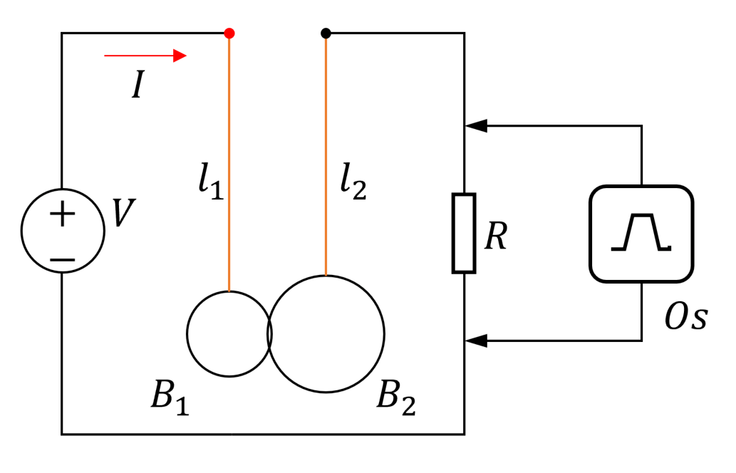
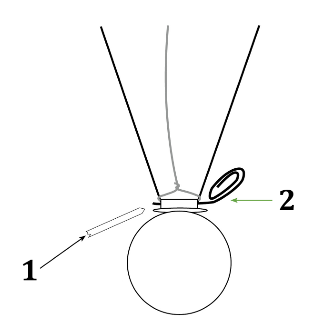
The Hertzian contact will last for a certain time and the balls will separate. In this part collision time ($\tau$) dependence on which parameters of the balls will be studied by making several collisions between same and different sized balls. To measure the contact time the electric circuit is used which is shown in Figure 6. Pendulum nylon wires are only for oscillation and additional thin metal wires connected to the balls. When you change the wires please make sure wires contacting the balls securely. To maintain this please use provided wooden toothpicks to lock metal wires and nylon wires without any slide through the ball hanger slot. Do not block both sides of the slot! To change the wires, you need to remove the locking toothpick pin. For this action the paper clip will be provided (Figure 7).

D.1 The collision time $\tau$ between the balls is given by the equation: $\tau = A \cdot x_1^{e_1} \cdot x_2^{e_2} \ldots \cdot x_n^{e_n}$ where $A$ is a dimensionless constant, and $x_1, x_2, \ldots, x_n$ (for some integer $n$) are physical parameters of the collision. Determine all of these physical parameters. The values of the exponents $e_1, e_2, \ldots, e_n$ will also be determined in parts D.2 and D.3.

D.2 By experiment, plot appropriate linear graphs to find the values of some exponents in the expression for $\tau$ in D.1.

D.3 Using dimensional analysis and the values of the exponents obtained in D.2, find the values of the remaining exponents.

D.4 Find the numerical value of $A$ with high accuracy (at least with 4 SF).

Part E: The parameters of Hertz deformation [3.0 points]

By using the equation of maximum speed in task A.2 and the experimental data based on task D.2, find the following parameters for a range of initial angles ($\nu = \nu_1 = \nu_2 = 0.3$, $E = E_1 = E_2 = 200$ GPa, $m_1 = 131.48$ g, $m_2 = 67.55$ g, $d_1 = 31.74$ mm, $d_2 = 25.42$ mm):

E.1 Find the expression and calculate the numerical value of average force $F_{av}$

E.2 Find the expression and calculate the numerical value of the Hertz deflection $\delta$

E.3 Expression and value of the Hertz radius $a$

E.4 Find the expression and calculate the numerical value of the Hertz pressure $P_0$

E.5 Find the expression and calculate the numerical value of the average pressure $P_{av}$

A.1 Find gradient (or slope) of $\Delta t^{-1}$ against $\sin\frac{\varphi_0}{2}$. Here $\varphi_0$ is the initial angle (or the angular amplitude) of the pendulum and $\Delta t$ is the time required for the fall to pass through the photogate. Remark 1. To measure time precisely on Digital storage oscilloscope, you are advised to follow oscilloscope instructions in the General Instructions (G). Beware of the model of your oscilloscope and instruction exercises. To save time you can make measurement for task B.1 together with this task. When the ball is released from electromagnetic holder, wire elasticity and magnetization of the ball may affect the initial speed of the ball. Therefore, you must not choose the first signal from the photogate.

D.4 Find the numerical value of $A$ with high accuracy (at least with 4 SF). [1,2 т.]

A.2 Derive the general equation to find maximum speed of the ball for any given initial angle of the pendulum. [0,2 т.]

B.1 Plot the linearized graphs of $T = f(\varphi_0)$ by measuring period of the oscillation. Note that different linearization, for appropriate regions, are required. Determine $T_0, \alpha, \beta$ from the graphs. Remark 2. To measure period very precisely on Digital storage oscilloscope, you are advised to do oscilloscope using exercises on the end of the Question sheets. Beware of model of your oscilloscope and instruction exercises. [1,6 т.]

B.2 By using gradient found in task A.1 and $T_0$ in task B.1 find the exact value of gravitational acceleration of Ulaanbaatar. The steel ball's diameter is $d = 31.75\ \mathrm{mm}$.

E.1 Find the expression and calculate the numerical value of average force $F_{av}$ [0,3 т.]

Решение

Оригинал в Архива: E1.pdf · официални решения: E1_sol.pdf