EuPhO 2020, Теория — Задача 1. Solenoid and loop
EuPhO-2020 Online — Theoretical Problems
Условие
A closed circular loop of radius consists of an ideal battery of electromotive force and a wire of resistance . A long thin air-core solenoid is aligned with the axis of the loop (-axis). Its length is , cross-sectional area is (), and the number of turns is . The solenoid is powered by a constant current provided by an ideal current source. The directions of the currents in the solenoid and in the loop are the same (clockwise in the figure).
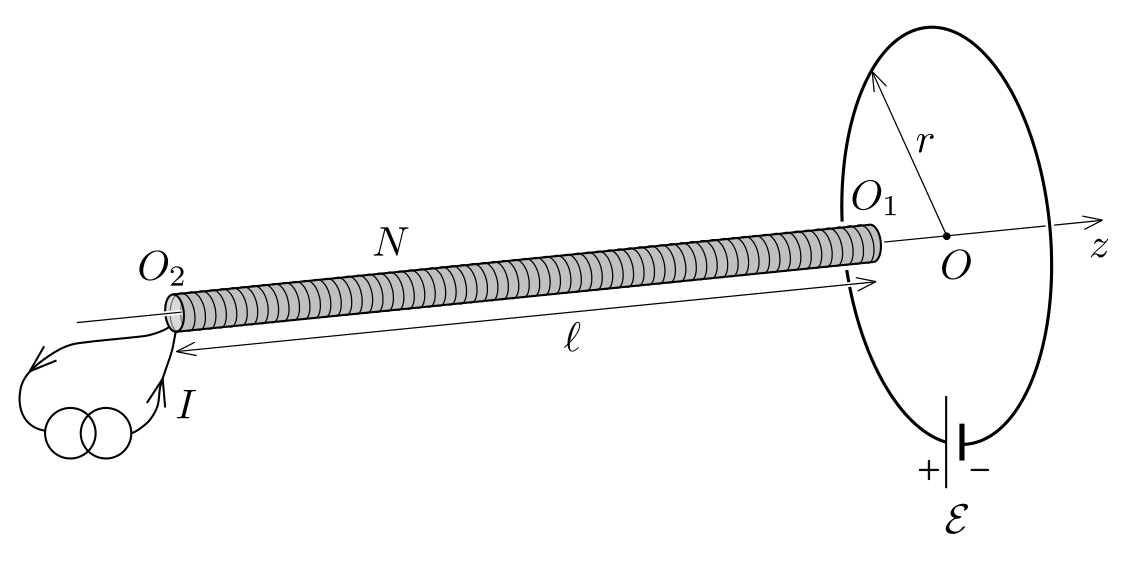
a. Find the force acting on the solenoid when its head is positioned in the loop centre . What is the force acting on the solenoid when its tail is located in the centre of the loop? [5,5 т.]
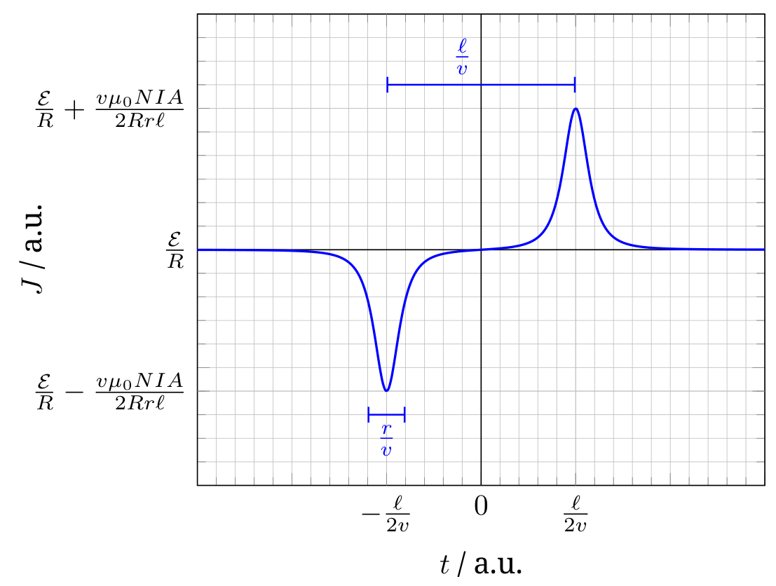
b. Suppose now, that the solenoid is moving slowly with a constant velocity along -axis starting far away from the loop, going past its centre, and proceeding further to the right in positive -direction. Plot the current flowing in the loop as a function of time. Highlight important features and values on the graph. The velocity is so small that self inductance of the loop can be neglected. [4,5 т.]
Отговори
a.
From the official solutions (Solution I–V for part a.).
b. J(t) = (ℰ + Vind(t))/R: a dip Jmin = ℰ/R − vμ₀NIA/(2Rrℓ) at t ≈ −ℓ/(2v), a peak Jmax = ℰ/R + vμ₀NIA/(2Rrℓ) at t ≈ ℓ/(2v), each of duration ~r/v; J ≈ ℰ/R elsewhere; J − ℰ/R is odd in t.
Решение
Part a. Solution I. According to Newton’s third law, the force acting on the solenoid is equal in magnitude, but opposite in direction to the force acting on the loop. The latter can be obtained from Lorentz’s law by summation of infinitesimal forces acting on the individual loop elements , where is the current in the loop.
Since the solenoid is long and thin, the magnetic field lines inside it are directed in direction, and escape only from the immediate vicinity of its ends. The magnetic field outside the solenoid is vortex-free and source-free. The same requirements are satisfied by the electric field in empty space. Hence, the magnetic field outside the solenoid can be well approximated by a field created by two magnetic poles: a North pole residing close to point and a South pole located near to . The flux emerging from the North pole (and the flux entering the South pole) is the same as the flux passing through the solenoid’s cross-section:
When the endpoint of the solenoid is placed in the loop centre , the magnetic field of the other end () near the loop is negligible. The field created by the North pole located at is pointing radially outwards, and its magnitude at the loop circumference is (from spherical symmetry):
Note. it is also correct to assume that the flux from the -field (which carries a factor of 1/2 compared to the field above at the end of the solenoid is uniformly distributed over hemisphere.
The forces acting on all elements of the loop (and also the net force) point in the direction, which can be expected also from the same current directions (i.e. the loop and the solenoid attract each other). Hence, the reaction force acting on the solenoid points in the direction, and its magnitude is given by:
When the endpoint is located at the centre of the loop, the magnetic field produced by the South pole exerts a force on the loop. Since this field is directed radially inward, the force acting on the solenoid is the same in magnitude, but opposite in direction () as the force calculated above:
| Grading scheme: T1 part a., Solution I. | |
|---|---|
| using Newton’s third law | 0.5 p |
| idea of approximating the outer field with magnetic poles 0.5 p, and justification 0.5 p | 1.0 p |
| calculating the flux emerging from the magnetic pole (for a wrong factor, 0.3 p) | 1.0 p |
| expressing the field of the magnetic pole | 1.0 p |
| finding the magnitude of force acting on the loop from Lorentz’s force law | 1.0 p |
| correct direction for 0.5 p, and antiparallel to 0.5 p | 1.0 p |
| Total for part a.: | 5.5 p |
Solution II. In this solution the force acting on the solenoid is calculated, as the force acting on the magnetic pole placed at the centre of the current-carrying loop. For this we need to find an expression for the magnetic pole strength (or magnetic charge) , which is defined as the ratio of the force and the magnetic field.
The total dipole moment of the solenoid is the product of the number of turns and the dipole moment of each turn:
This can be also expressed with the magnetic pole strength and the distance of the poles: . From this we arrive to the expression
where is the total flux emerging from the pole (see solution I).
Note. The same result can be obtained from the analogy between electrostatic and magnetostatic fields. The Coulomb force between two point charges can be derived from the principle of virtual work. The force is the derivative of the interaction part of the field energy with respect to the distance between the charges. The force between two magnetic charges can be also calculated this way. From the expressions of electric and magnetic energy densities we can conclude the formula of the magnetic interaction force:
As it can be seen, the well-known formulae known in electrostatics can be also used in magnetostatics with the substitutions , , . Carrying on this analogy the magnetic pole strength can be figured out:
where and are the electric and magnetic flux for a closed surface containing the electric and magnetic charge, respectively.
When endpoint of the solenoid is located at point , a North pole resides at the centre of the loop. Here the magnetic field created by the loop can be expressed from Biot–Savart-law:
pointing in the direction. So the magnitude of the force acting on this end of the solenoid is:
and it is directed to . When the endpoint is located at the center of the loop, the force acting on the South pole should be calculated, resulting a force of same magnitude, but opposite direction.
| Grading scheme: T1 part a., Solution II. | |
|---|---|
| idea of approximating the outer field with magnetic poles 0.5 p, and justification 0.5 p | 1.0 p |
| calculating the magnetic pole strength (for dimensionally wrong answer 0 p) | 1.0 p |
| justification for calculation | 1.0 p |
| calculating the field of the current loop at its centre from Biot–Savart-law | 0.5 p |
| finding the magnitude of force acting on the magnetic pole | 1.0 p |
| correct direction for 0.5 p, and antiparallel to 0.5 p | 1.0 p |
| Total for part a.: | 5.5 p |
Solution III. Some of the magnetic field lines created by the loop enter into the near end of the solenoid; this entering flux is given by
Since the end is far from the loop, the flux created by the loop escaping there is negligibly small. This means that almost all the flux escapes from the solenoid through its side.
Denote the radial component of the magnetic field vector produced by the current-carrying loop at the perimeter of the th turn of the solenoid by . Only this component contributes to the net force acting on the solenoid, as the axial component produces a radial force which is cancelled due to rotational symmetry. The axial force acting on the th turn of the solenoid is given by
where is the circumference of one turn, and the force points in the direction. Summing up both sides gives the net force:
Take out the factor from the summation and insert written in the unusual way :
The sum on the right hand side is the flux escaping through the side of the solenoid, which equals , so the force:
which agrees with the previous solutions.
| Grading scheme: T1 part a., Solution III. | |
|---|---|
| -field at the center of loop | 0.5 p |
| expressing force on one turn | 1.0 p |
| realizing that all the flux escapes through the sides of the solenoid | 0.5 p |
| relating the force to escaping flux | 1.5 p |
| summation and correct result | 1.0 p |
| correct direction for 0.5 p, and antiparallel to 0.5 p | 1.0 p |
| Total for part a.: | 5.5 p |
Solution IV. The force acting on a current loop of magnetic moment placed in magnetic field is given by . Divide the solenoid into short circular coils of equal length , then the magnetic moment of each short coil is
where denotes the unit vector in -direction. This magnetic moment is parallel to the field created by the large current-carrying loop, so the force acting on each short segment of the solenoid in -direction can be written as:
The total force on the solenoid can be determined from integration of the force contributions along the solenoid:
Using the Biot–Savart-law we can compute the magnetic field of the current-carrying loop along the -axis to
This expression for yields
and is directed to . From a similar calculation we get .
| Grading scheme: T1 part a., Solution IV. | |
|---|---|
| idea of dividing the solenoid into short segments of equal lengths | 1.0 p |
| giving the magnetic moment of a segment | 0.5 p |
| expressing the force on a segment by a derivative of the magnetic field | 1.0 p |
| calculating the field of the current-carrying loop from Biot–Savart-law (alternatively, arguing that only the field at center of loop is important 0.5 p and calculating this field 0.5 p) | 1.0 p |
| integrating force contributions to find total force on solenoid (max. 0.5 if final expression still contains integral) | 1.0 p |
| correct direction for 0.5 p, and antiparallel to 0.5 p | 1.0 p |
| Total for part a.: | 5.5 p |
Note: Using the idea of dividing the solenoid into small segments other solutions are possible as well (e.g. considering small dipole contributions). In this case the grading scheme of Solution IV should be adapted accordingly. One recurring solution of this type is to divide the solenoid into small segments of length , compute the -field in -direction effected by current-loop from Biot–Savart, use Gauss law to relate the radial -flux through the segment to . compute the force on the segment using Lorentz forces and integrate the force over the length of the solenoid. In this case the marking scheme is adapted in the second aspect, awarding 0.5 p for the idea of using Gauss law to find radial -field
Solution V. In this solution we relate the force acting on the solenoid to the change in energy of the system. Investigate the case when point is located at first. Due to the same current directions, the magnetic force acting on the solenoid points in direction . While keeping the solenoid in equilibrium with external force , let it move by a small displacement in the positive direction. The work done by the external force is equal to the change in energy of the system:
We should be aware of the fact that the system is not closed: there is also a battery and a current source included in the circuits. Hence, contains the change in field energy and the change of energy of the power sources:
Since the force does not depend on what kind of power supplies we have, let us replace the battery with a current source providing constant current .
Now we find a relation between and The energy stored in the field can be expressed as
where is the inductance of the solenoid, is that of the loop and is the mutual inductance of the system. Upon small displacement , only the last term changes, so
The small displacement results in a change of the flux enclosed by the loop and the solenoid. The flux created by the solenoid on the loop is , and the flux created by the loop through the solenoid is (here we used the symmetry property of mutual inductance). During the short time of the displacement , the e.m.f. induced in the loop () and the solenoid () can be expressed with Faraday’s law:
In order to keep the current in the circuits constant, the current sources need to provide an additional power, so they give away extra energy (in addition to Joule heat). This energy change of the sources is given by:
Using the previous results we finally get:
which means , and hence .
Note 1. Naively, one might think that we get the result if we imagine superconducting wires without power supplies. One can show with detailed calculation that in that case the currents in the loop and the coil change, as the total flux enclosed by a superconducting circuit must remain constant. The correct physical justification of the appearing negative sign is an important part of the solution.
Now we calculate the change in mutual inductance . The small displacement can be imagined as we take a short segment from the tail of the coil (consisting of turns) and move it to the head . As a result, the flux produced by the loop on the solenoid increases by
From this we get:
If the tail of the solenoid is located at point , the coefficient of mutual inductance decreases upon small displacement, which results in .
Note 2. The field energy can be also calculated from the energy density integrated for the whole space. Instead of calculating the total field energy, it is easier to find its change using the same idea presented above, i.e. take a segment of length from the tail and move it to the head of the solenoid. Assuming , the field created by the solenoid inside that segment is (because the field differs from this only at distance from the ends). At the end we get the same result for the change in field energy using the expression:
Note 3. A third possibility is to calculate the potential energy change of the displaced few turns of the solenoid. The magnetic moment of a segment of length is , and its energy in external field is . Important to highlight that this potential energy already contains the factor of discussed at the beginning of the solution, so the force acting on the solenoid can be expressed as
The external field is the superposition of the field created by the loop and the field created by the coil (note that this latter contains a factor of compared to the field in the middle of the solenoid). Since is the same at the two ends and , the energy change is:
The second term can be neglected, and we get
which gives the same answer for as the other ideas.
| Grading scheme: T1 part a., Solution V. | |
|---|---|
| Equating force to energy change in system | 0.5 p |
| Formulating energy equation (if sources are missing 0.2 p) | 0.5 p |
| expressing through contributions from currents and an interaction term | 1.0 p |
| deriving that | 1.0 p |
| computing the change in field energy and final result for force. | 1.5 p |
| correct direction for 0.5 p, and antiparallel to 0.5 p | 1.0 p |
| Total for part a.: | 5.5 p |
Part b. In order to plot a graph displaying the important features, it is beneficial to make some calculations. The problem text does not specify the zero point of time, so take in the moment when the center of the solenoid is located at point . This means that at time the head of the solenoid is located at , while the tail is located at .
The current flowing in the loop at an arbitrary moment of time is given by
where is the induced electromotive force in the loop as a function of time. Two different approaches can be found below which give an analytical formula for this induced e.m.f.
Solution I. We may again approximate the magnetic field outside the solenoid by a field created by two magnetic poles at and , respectively. The resulting magnetic flux through the loop can be calculated by considering the solid angle the loop extends as seen from either of the poles. Using the total magnetic flux of the poles as calculated in Solution I for part a. we get
Using this result and the induced e.m.f. can be calculated with Faraday’s law , which gives
Solution II. The rate of change of flux produced by the solenoid through the loop can be expressed in terms of the mutual inductance of the solenoid with respect to the loop:
Using the symmetry property of mutual inductance (), instead of calculating let us find the time derivative of , i.e. the mutual inductance of the loop with respect to the solenoid. For this, imagine that the current in the loop is constant , and calculate the change of flux produced by the loop through the solenoid during a short amount of time ! The small displacement of the solenoid can be considered as moving a short segment of length from the tail to the head. The change in flux in this segment is given by
Using the formula for obtained from Biot–Savart-law (see Solution IV for part a.) we get
From this the induced e.m.f. can be expressed:
Although the analytical result gives the correct expression for the current flowing in the loop, the task in part b. was to plot the graph.
The graph should reflect the most important features of the function. First, is an odd function, i.e. . For the flux through the loop increases meaning that and , while for the flux decreases, which results and .
In different ranges of time, behaves very differently. For times and the solenoid is very far (approximately at distance ) from the current loop, and its field can be approximated by dipole field (proportional to ). The time derivative of the field is proportional to the induced e.m.f. in the loop, so in this time range , and has very small value. The same result can be concluded from the Taylor expansion of the complete analytical formula for .
When (with the accuracy of ) the effect of one pole of the solenoid can be neglected. The absolute value of the induced e.m.f. is maximal here:
so the maximal and minimal value of the current are
Around the maximum is a quadratic function of time, as it can be proved with expanding the complete analytical formula.
When the centre of the solenoid is close to the centre of the loop, i.e. , the flux barely changes, so . A more careful analysis gives a very weak linear dependence on time.
The statements above are summarized in the table below.
| time range | ||
|---|---|---|
| small, | ||
| large, | , dip | |
| negligible () | ||
| large, | , peak | |
| small, |
| Grading scheme: T1 part b. | |
|---|---|
| relating to or other suitable quantity (independent of result in a.) | 0.5 p |
| the graph is smooth everywhere (if graph does not capture whole domain including asymptotics, 0 p.) | 0.5 p |
| , except if (if only asymptotically, 0.2 p) | 0.5 p |
| is clearly an odd function (computing analytical expression for and graph showing odd behavior is considered sufficient, if reasoning is missing, 0.2 p) | 0.5 p |
| has a minimum first, then a maximum time later (if reversed or the time is incorrect, 0 p) | 1.0 p |
| analytical formula for and (either approximate or exact), if analytical expression is given but min-max values are not determined 0.5 p are given for deriving the formula and realizing that min-max exist. | 1.0 p |
| it is indicated that the duration of the peak and dip is in the range of | 0.5 p |
| if instead of is plotted or labels are missing on the axes 0.5 p are deducted from part b. but only if 0.5 or more marks are given to the actual graph at all | (-0.5 p) |
| Total for part b.: | 4.5 p |
If no graph is drawn: max. 0.5 p for relating to and 1.0 p for and (for a general formula without evaluation of min and max: 0.5 p) are given.
If -field of the solenoid is assumed constant across loop or area for flux is taken to be , 0 p are awarded for min and max.
Additional general guidelines for grading T1:
- Grading should always follow one of the solutions described. If approaches for solutions are mixed the one resulting in the highest marks is considered.
- Granularity for marks is 0.1 p.
- A simple numerical error resulting from a typo is punished by 0.1 p unless the grading scheme explicitly says otherwise.
- Errors which cause dimensionally wrong results are punished by at least 50 % of the marks if dimensions can easily be checked. In more complicated cases less marks may be deducted.
- Propagating errors are not punished repeatedly unless they either lead to considerable simplifications or wrong results whose validity can easily be checked.
- No marks are given for the directions of the forces in a. if forces are physically incorrect (e.g. resulting force is calculated to zero) or if no forces are calculated.
- If current in solenoid is used as current in loop instead of or vice versa in the calculation of the force 0.5 p are subtracted.
- If only -component of -field (either from solenoid or loop) is determined and the force on the solenoid is derived from this using Lorentz-forces, marks are only given for ideas (max. 1.0 p.) and the use of the Biot–Savart law (max. 1.0 p)
Оригинал в Архива: EuPhO_2020_Theory.pdf · официални решения: EuPhO20_Theory_Solutions-7.pdf