Съдържание

EuPhO 2021, Експеримент — Задача 2. E2: Hot Cylinder

Оригинал на условието (PDF)Съобщи за грешка

Всички материали от EuPhO 2021

EuPhO-2021 Experimental problems. Language: English

Условие

Introduction

A uniform metal rod of length $L = 30\ \mathrm{cm}$ and radius $r = 1\ \mathrm{cm}$ is made of an unknown metal and is kept at room temperature $T_0 = 26.9\ \mathrm{C} = 300\ \mathrm{K}$ . The metal rod is weighed to be $m = 460\ \mathrm{g}$ . Your task is to determine the thermal properties of the unknown metal. The metal rod can be heated at one of its ends, and temperature measurements can be performed on customizable locations along the rod. The heater is located between $x = 0$ and $x = L_h = 3\ \mathrm{cm}$ (see fig). The heater can be programmed by specifying a fixed power (in watts) and the duration (in seconds) for which the heater is turned on for. Temperature measurements are made by specifying up to five locations for the sensors along the rod, alongside with the frequency, starting time and the ending time of the measurements. The simulation will show the temperature readings in accelerated ”real time” (running around 10 times faster than in the real world).

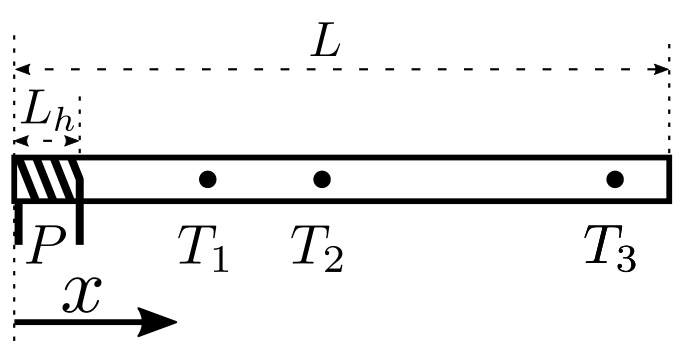
Horizontal rod of length L with the heater section of length L_h at the left end (hatched, labelled P); three temperature sensor points T1, T2, T3 along the rod; an arrow labelled x pointing to the right from the heated end.

You may assume that all of the heating power goes into the rod, and that the rod loses heat to its surroundings via heat transfer with air and black body radiation. Heat transfer with air is linear in temperature of the rod, and can be described by a coefficient $\alpha$ such that the heat transfer per unit area per unit time is $\alpha(T - T_0)$ . The air is well-ventilated such that $\alpha$ can be assumed to be constant throughout the surface of the rod and independent of the temperature of the surface. Heat loss via black body radiation can be described using the Stefan-Boltzmann law modified with emissivity $\beta$ such that the heat loss to radiation per unit area per unit time is $\beta\sigma(T^4 - T_0^4)$ where $\sigma = 5.67 \times 10^{-8}\ \mathrm{W/(m^2\,K^4)}$ . Similar to $\alpha$ , the emissivity can be assumed to be constant throughout the rod, and independent of temperature. The rod is further characterised by the thermal conductivity $k$ (such that the heat flux density along $x$ is $-k\mathrm{d}T/\mathrm{d}x$ ) and the specific heat capacity $c$ .

Task

The task is to determine the specific heat of the unknown metal, $c$ (units $\mathrm{J/(K\,kg)}$ ), the thermal conductivity $k$ (units $\mathrm{W/(m\,K)}$ ), and the heat loss coefficients $\alpha$ (units $\mathrm{W/(m^2\,K)}$ ), and $\beta$ (dimensionless). You should aim to find the values within 10 % of the true value. This is because there are various sources of errors, such as Gaussian fluctuations in both defining the locations of the sensors, and the taking the temperature measurements. The sizes of the errors can be found by observing the fluctuations in the output.

As with all experiments, you must provide clearly labelled tables of data, clearly labelled graphs, and sufficient formulae derivations to make it clear what you have measured, and how you are deriving your results.

Program interface

Running the simulation program, named rod, allows performing multiple experiments on the rod. The program will ask a sequence of prompts regarding the setup of the experiment. For each prompt, the corresponding value(s) should be entered, followed by pressing return to go the next prompt. The prompts are as follows:

The heating power of the heater:

Enter P (W), between 0 and 300: 2. The duration after the start of the experiment for which the heater is turned on for (after this time, the heater will be turned off):
Enter heating duration (s), between 0 and 3600s: 3. The starting and finishing times (after the start of the experiment) for the temperature measurements made on the rod:
Enter the starting and finishing time for the measurements (s), separated by a space. Must be between 0 and 3600s: 4. The time interval between two consecutive measurements that are made with the temperature sensors:
Enter dt (s), between 5 and 3600s and a multiple of 5s: 5. The locations of the temperature sensors along the rod. The coordinates are specified with respect to the end with the heater:
Enter up to 5 locations for the sensors (in cm), between L=0 and L=30cm, separated by spaces:
Note that not entering any numbers simply means not taking any measurements. 6. The output file name for the temperature readings. Note that all of the saved readings will also be displayed on the screen:
Enter the output file name:
You are advised to only use Latin letters and numbers for the name. Other characters may or may not be allowed in the filename and in case of an invalid filename, the readings will not be saved. The readings will be saved in a .txt file with the given name in the same folder as the program.

If you enter an invalid input, a clarifying error message will be sent, and an another opportunity for entering the input will be given.

The program will then prompt to press return to start the experiment, or typing restart and pressing return to re-enter all the experimental parameters. After continuing with the simulation, the program will display a summary of the experimental setup, and then start printing out the time elapsed since the heater was turned on (t(s)), and all the sensor readings in the same order they were entered in the prompt (Ti(C), where i corresponds to the i-th sensor).

After the simulation ends, a new experiment can be started by typing restart and pressing return.

Отговори

Решение

Start the experiment with the heater on full for 300 Watts and the thermostats located evenly across the length of the rod and display the results every 100 seconds. Then plan out the remainder of the experiment while waiting, or do the other experiment. The rod reaches steady state at about 600 seconds. Find the average temperature at the five thermostats by considering the last five measurements; you will use this later.

The most accessible approach is then to study the steady state behavior, the uniform temperature behavior, the low temperature behavior, and the high temperature behavior. Separating the low and high temperature behaviors is useful because blackbody radiation dominates at higher temperatures while convective loss is most significant at near room temperature.

Finding the heat capacity is done by heating the rod at a low enough rate for a short enough time so that heat loss is as small as possible.

One possibility is to give a total of 1500 J of heat, but at various power settings and various times, while keeping the temperature as low as possible.

The average temperature of the rod is computed from the five equally spaced points by applying Simpson's rule,

T_{avg} = \frac{T_1 + 4T_2 + 2T_3 + 4T_4 + T_5}{12}

Computing instead a direct average yields a $+5$ % error.

It is found that the average temperature for heating times less than 50 seconds is $55.4{\pm}0.5$ °C, yielding specific heat capacity of $c = 114 \pm 1$ J/kg K.

Heat the rod full power for 600 seconds, and then allow to cool.

The rod temperature becomes uniform at about 700 seconds. Average the five points to obtain an average rod temperature.

Linear cooling predicts a straight line graph for $\ln(T - T_0)$ versus $t$

The convective heat loss rate is then given by $A\alpha(T - T_0)$ , where $A$ is the surface area of the rod. Do not forget the end caps!

The radiative heat loss rate is $\beta\sigma(T^4 - T_0^4)$ where $\sigma = 5.67 \times 10^{-8}\ \mathrm{W/(m^2\,K^4)}$ . The radiative heat loss rate is then given by $A\beta\sigma(T^4 - T_0^4)$ .

Note that at temperatures close to $T_0$ the radiative expression can be written as

A\beta\sigma(T^4 - T_0^4) \approx A\beta\sigma 4(T - T_0)T_0^3

This means that the linear heat loss rate at temperatures close to $T_0$ is

A\left(\alpha + \beta\sigma 4T_0^3\right)(T - T_0)

For the uniform, low temperature cooling rod,

mc\frac{\mathrm{d}T}{\mathrm{d}t} = -A\left(\alpha + \beta\sigma 4T_0^3\right)(T - T_0)

The solution is of the form

T - T_0 = Ce^{-Bt}

where

B = A\frac{\alpha + \beta\sigma 4T_0^3}{mc}

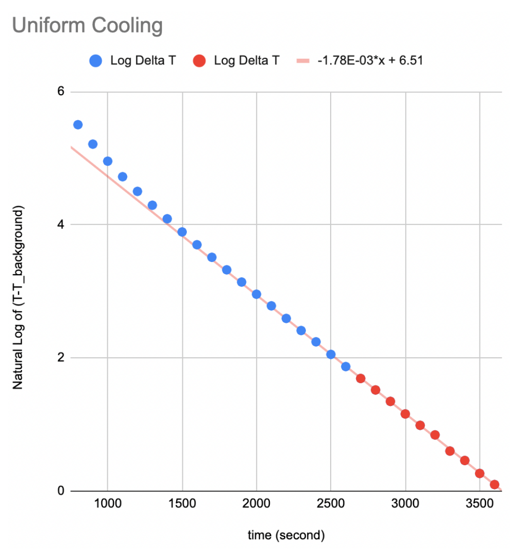
On a log plot of $\ln(T - T_0)$ as a function of time $t$ , the plot should be linear, with a slope given by

-A\frac{\alpha + \beta\sigma 4T_0^3}{mc}

It is also possible to plot $\mathrm{d}T/\mathrm{d}t$ as a function of $T - T_0$ , and the plot will be linear, with a slope also given by

-A\frac{\alpha + \beta\sigma 4T_0^3}{mc}

The slope in either case is found to be $-1.78 \times 10^{-3}$ /s.

Chart titled Uniform Cooling: Natural Log of (T-T_background) from 0 to 6 versus time (second) from about 800 to 3600; blue points (Log Delta T) fall along a curve, red points (Log Delta T) at later times lie on a pink fitted line labelled -1.78E-03*x + 6.51. — Uniform Cooling. Note that only the last points (in red) were used to determine the linear cooling line. It is clearly a good fit from $t = 2000$ s on, which corresponds to rod temperatures of $T < 45$ C.

To find the blackbody behavior we want to heat the rod as much as possible such that the blackbody heating becomes the dominant form of heat loss. Since the hot rod is in steady state, the heat radiated must be equal to 300 W. Use the results from the beginning.

The average temperature of the rod is computed from the five equally spaced points by

T_{avg} = \frac{T_1 + 4T_2 + 2T_3 + 4T_4 + T_5}{12} = 662\ \mathrm{°C}.

Computing a direct average yields a $+1.5$ % error.

The average of $T^4$ is found from

T^4_{\mathrm{avg}} = \frac{{T_1}^4 + 4{T_2}^4 + 2{T_3}^4 + 4{T_4}^4 + {T_5}^4}{12} = 7.95 \times 10^{11}\ \mathrm{K}^4

Computing a direct average yields a $+6.3$ % error.

The rate of linear temperature heat loss is found from above to be

(-1.78 \times 10^{-3}\ /\mathrm{s})mc\Delta T = 59\ \mathrm{W}

The blackbody remainder term is then

300 - 59 = 241\ \mathrm{W},

and necessarily equals

A\beta\sigma(T^4 - T_0^4) - A\beta\sigma 4T_0^3(T - T_0),

where the second term reflects the fact that we had considered part of the blackbody behavior as being linear.

Solving, $\beta = 0.304 \pm 0.004$ .

Failing to subtract the second term would yield $\beta = 0.28$ .

We are now in a position to find $\alpha$ , from

-A\frac{\alpha + \beta\sigma 4T_0^3}{mc} = -1.78 \times 10^{-3}\ /\mathrm{s}

which yields $\alpha = 2.93$

Alternatively, for the uniform, high temperature cooling rod,

mc\frac{\mathrm{d}T}{\mathrm{d}t} \approx -A\beta\sigma\left(T^4 - T_0^4\right)

as the radiative cooling effect will dominate.

On a plot of $\mathrm{d}T/\mathrm{d}t$ as a function of $T^4 - T_0^4$ , the plot should be linear, with a slope given by

-\frac{A\beta\sigma}{mc}

The slope is found to be $-7.8 \times 10^{-12}\ \mathrm{K^3/s}$

This means $\beta/c = 3.25 \times 10^{-3}$ kg K/J; this gives $\beta = 0.36$ , which is too high; ignoring the linear loss effects was significant; as was previously seen, almost 20% of the heat loss is from convection in this temperature range.

We can use the high temperature behavior to find the heat flux through the center of the rod. The average of $T$ and $T^4$ on the non-heated half of the rod is $599$ C and $5.8 \times 10^4$ K $^4$ , yielding a heat loss at $112$ W. That heat necessarily came from the other side of the rod.

The temperature gradient is $-898$ K/m, so $k = 397$ W/mK. Don't forget that the formula provided gave the rate of heat flux, which means that we needed to consider the cross sectional area of the wire.

Marking scheme

Finding $c$ , 2.5 pt total

	Task	Pts
2.1	Idea of heating the rod by a fixed $Q$ .	0.6
2.2	Obtaining an equation relating the inserted heat with the temperature change and $c$ .	0.4
2.2	Heating the rod for a short duration for mitigating the effects of heat loss:
	heating for less than 60 seconds.	0.2
2.3	Averaging the temperature of the rod:
	averaging over one to three points;	0.1
	Use Simpson rule (or equivalent)	0.3
	averaging over four or more points;	0.2
2.4	Checking more than one time value	0.2
2.5	Numerical value of $c$ :
	$c$ within [103;123] J/(K kg);	0.3
	$c$ within [108;118] J/(K kg).	0.2

Finding the linear heat loss, 2.0 pt total

	Task	Pts
3.1	Idea of looking at how the rod cools down at the low temperature limit (with no heating).	0.2
3.2	Obtaining an equation for $T$ as a function of $t$ in terms of $\alpha$ , $\beta$ , and $c$ :
	linearize radiative loss around $T_0$ ;	0.3
	obtaining a differential equation for $T(t)$ ;	0.1
	solving the differential equation to get $T(t)$ .	0.2
3.3	Finding the average temperature at $t$ :
	averaging over one to three points;	0.1
	Use Simpson rule (or equivalent)	0.3
	averaging over four or more points;	0.1
3.4	Graphically finding the slope (which is a function of $\alpha$ , $\beta$ , and $c$ ):
	Plot 2 to 4 points in range $T < 50$ C;	0.1
	Plotting 5 or more points in range $T < 50$ C;	0.1
	axes labels and units;	0.1
	axes tickmarks with values.	0.1
3.5	Numerical value of the slope:
	slope within $[-1.58 \times 10^{-3}, -1.98 \times 10^{-3}]$ ;	0.2
	slope within $[-1.68 \times 10^{-3}, -1.88 \times 10^{-3}]$ ;	0.1

Finding $\beta$ , 2.5 pt total

	Task	Pts
4.1	Idea of looking at the steady state at the high temperature limit.	0.2
4.2	Writing down the heat balance:
	accounting for the area of the end caps;	0.1
	accounting for the linear contribution to the heat loss by removing the $\alpha$ dependence from the previously found slope;	0.2
	final expression for $\beta$ in terms of mean value of $T$ and $T^4$ of the steady state. Making a mistake in the previous parts shouldn't be penalised here.	0.2
4.3	Measurements:
	Heating power sufficiently big such that the steady state temperature is bigger than 500 °C;	0.1
	Waiting for at least 300s to reach the steady state	0.1
	Waiting for at least 600s to reach the steady state	0.1
4.4	Finding the average temperature:
	averaging over one to three points;	0.1
	Use Simpson rule (or equivalent)	0.3
	averaging over four or more points;	0.1
4.5	Finding the average $T^4$ (for calculating average radiative loss):
	averaging over one to three points;	0.1
	Use Simpson rule (or equivalent)	0.3
	averaging over four or more points;	0.1
4.6	Numerical value of $\beta$ :
	$\beta$ within [0.25;0.35];	0.3
	$\beta$ within [0.28;0.32].	0.2

Finding $\alpha$ , 0.5 pt total

	Task	Pts
5.1	Obtaining an expression for $\alpha$ in terms of the slope $\gamma$ .	0.1
5.2	Numerical value of $\alpha$ :
	$\alpha$ within [2.33;3.23]W/(m $^2$ K);	0.2
	$\alpha$ within [2.53;3.03]W/(m $^2$ K).	0.2

Finding $k$ , 2.5 pt total

	Task	Pts
6.1	Idea of looking at the flux from part of the rod to the other	0.4
6.2	Theory:
	Expressing heat flux in terms of $k$ and the temperature gradient;	0.2
	Expressing heat flux in terms of the average $T$ , $T^4$ , and the heating power of one of the halves of the rod;	0.4
	accounting for the area of the end caps.	0.1
6.3	Finding the average temperature of one of the halves:
	averaging over one to three points;	0.1
	averaging over four or more points. No marks if points not equally spaced and average doesn't account for the unevenness;	0.1
6.4	Finding the average $T^4$ (for calculating average radiative loss):
	averaging over one to three points;	0.1
	averaging over four or more points;	0.1
6.5	Finding the temperature gradient:
	Using at least two points for the gradient calculation;	0.1
	Using $(f(x + h) - f(x - h))/2h$ for numerical derivative;	0.2
	Having the range of points used for gradient calculations not farther apart than 5 cm;	0.1
	Having the range of points used for gradient calculations not closer than 1 cm;	0.1
6.5	Numerical value of $k$ :
	$k$ within [328;488]W/(m K);	0.3
	$k$ within [378;438]W/(m K).	0.2

Some grading notes:

Failure to record and report the location of the sensors will result in a penalty of -1.0 pt for each occurrence!. It is acceptable to clearly state the location of the sensors in one part of the report, and then mentioning that they are not moved during the experiment.
When computing spatial averages, if the spacing between thermometers is not uniform, the averaging techniques must use appropriate weighting, or there is a penalty of -0.1 pt for each occurrence!
When computing spatial averages, if the rod is not mostly uniform in temperature, a Simpson's Rule technique or equivalent must be used to obtain the 0.3 pts. If instead all of the temperatures are within two error limits, then Simpson is not required to obtain the 0.3 pt.
Any numerical derivatives must use the symmetric form

f'(x) \approx (f(x + h) - f(x - h))/2h

or some equivalent, or better, method.

Оригинал в Архива: EuPhO_2021-exp.pdf · официални решения: EuPhO_2021_exp_solutions-2.pdf