Съдържание

GPhO 2019, Експеримент — Задача 1. Problem E1. Magnetic properties of matter

Оригинал на условието (PDF)Съобщи за грешка

Всички материали от GPhO 2019

The 3rd Gulf Physics Olympiad — Experimental Competition. Muscat, Oman — October 8th 2019 · 8 октомври 2019 г. · 20 т.

Корица

The examination lasts for 5 hours. There is one problem worth in total 20 points.
Initially the experimental equipment on one table is covered. You must neither remove the cover nor open the envelope with the problems before the sound signal of the beginning of competition.
You are not allowed to leave your working place without permission. If you need any assistance (malfunctioning equipment, broken calculator, need to visit a restroom, etc), please raise and keep your hand raised until an organizer arrives.
Use only the front side of the sheets of paper.
For each problem, there are dedicated Solution Sheets (see header for the number and pictogramme). Write your solutions onto the appropriate Solution Sheets. For each Problem, the Solution Sheets are numbered; use the sheets according to the enumeration. Always mark which Problem Part and Question you are dealing with. Copy the final answers into the appropriate boxes of the Answer Sheets. There are also Draft papers; use these for writing things which you don’t want to be graded. If you have written something what you don’t want to be graded onto the Solution Sheets (such as initial and incorrect solutions), cross these out.
If you need more paper for a certain problem, please raise your hand and tell an organizer the problem number; you are given two Solution sheets (you can do this more than once).
You should use as little text as possible: try to explain your solution mainly with equations, numbers, symbols and diagrams. Though in some places textual explanation may be unavoidable.
After the signal signifying the end of examination you must stop writing immediately. Put all the papers into the envelope at your desk. You are not allowed to take any sheet of paper out of the room. If you have finished solving before the final sound signal, please raise your hand.

Error analysis

In what follows, any time errors of the mean of tabulated data are calculated, standard deviation is used. Assuming there are $N$ data points of the form $x_i$ , $i \in \{1, \ldots, N\}$ , the mean is

x_{\mathrm{avg}} = \frac{1}{N}\sum_{i=1}^{N} x_i,

and the standard deviation of the mean

\Delta x_{\mathrm{avg}} = \sqrt{\frac{\sum_{i=1}^{N}(x_i - x_{\mathrm{avg}})^2}{N(N-1)}}.

For error propagation through equations, Pythagoran rule for adding errors in quadrature is used (alternatively, one could use min-max but for lower accuracy). In general, when you have a variable $y$ be a function of variables $x_i$ , $i \in \{1, \ldots N\}$ with errors $\Delta x_i$ , then the error of $y$ is given by

\Delta y = \sqrt{\sum_{i=1}^{N}\left(\frac{\partial y}{\partial x_i}\right)^2 \Delta x_i^2}.

Any time the methods used in finding the errors is not specified, $50\,\%$ of the marks for error analysis are to be deducted.

Условие

The aim of this experiment is to measure magnetism-related characteristics of dia- and ferromagnetic materials. To reach this goal, some other measurements are also required — e.g. measuring the diameter of the syringe needle, and the coefficient of surface tension of water.

Equipment

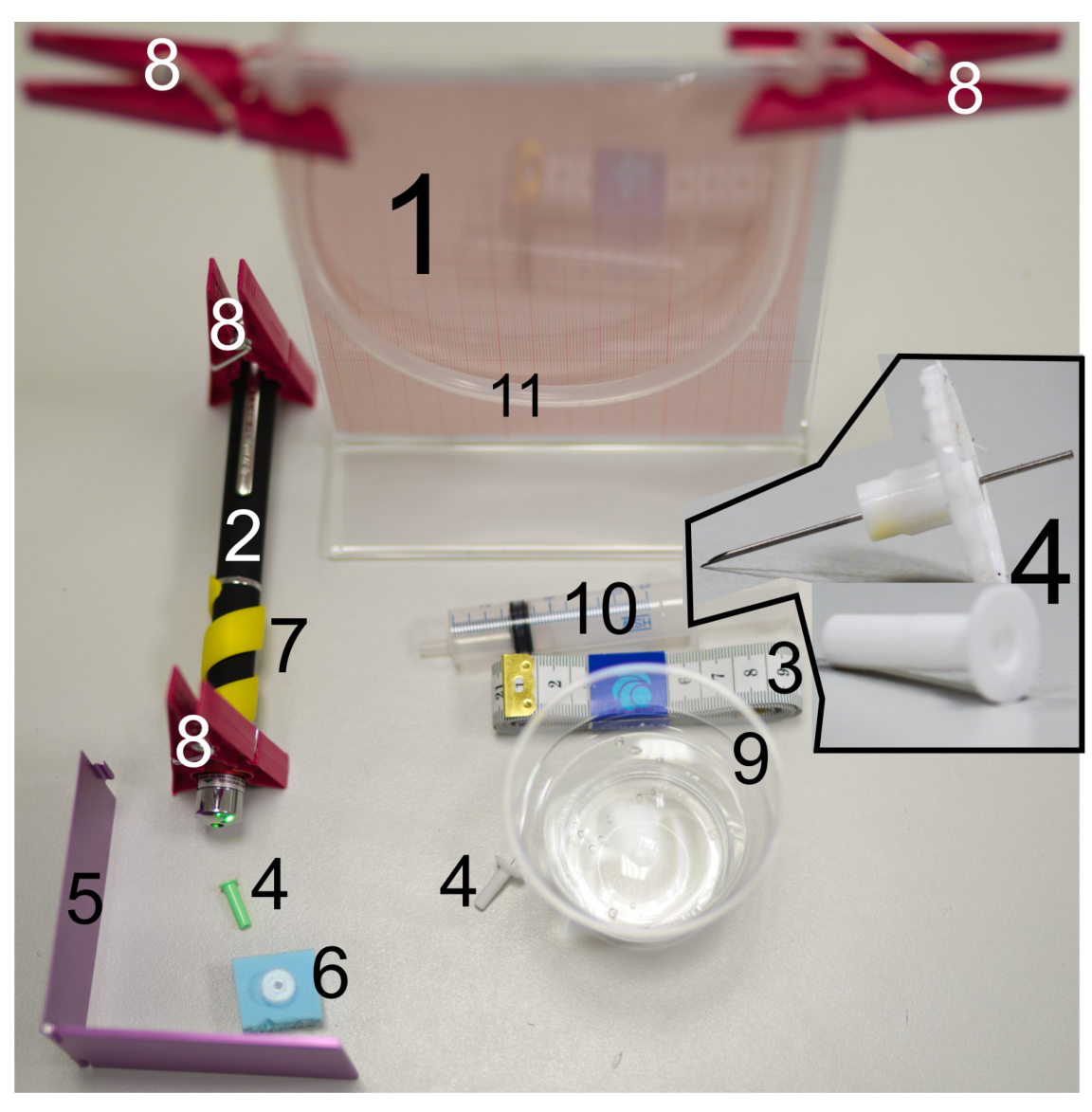
Photo of a Petri dish (1) with a graphite bar (3) lying in it, above a ruler (2) graduated 0–12 cm. — Figure 2

Photo of the magnetic equipment with numbered labels: 1 stand-alone ferromagnetic strip, 2 reinforced strip with measuring tape, 3 wires with crocodile clips, 4 batteries, 5 battery holder (insert shows its + and − leads), 6 multimeter, 7 magnetic field sensor (circled), 8 plastic clamp, 9 magnet (circled), 10 plastic spacer (circled); an insert shows the magnet 9 between strips 1 and 2. — Figure 3

The following equipment is listed in figure 1:

1 — a stand;

2 — green laser pointer

3 — a measuring tape;

4 — green and white syringe needles, one end of the needle is sharp, and the other end is cut perpendicularly to its axis, see the insert in fig 1

5 — a foldable mirror

6 — a piece of foam

7 — a spiral plastic fixator that keeps the laser pointer button pressed;

8 — clothespins;

9 — a cup with water;

10 — a syringe;

11 — a silicone tube,

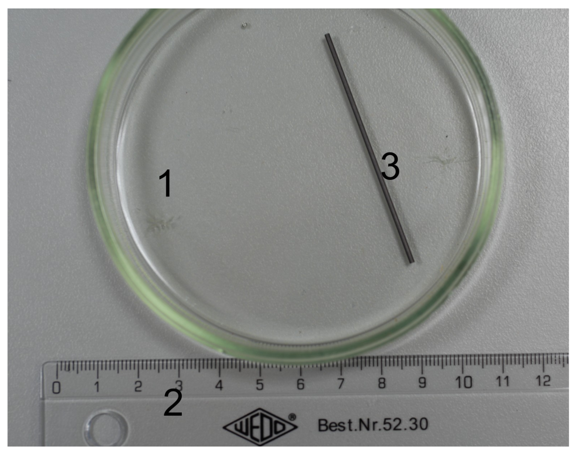
The following equipment is listed in figure 2:

1 — a Petri dish;

2 — a ruler;

3 — a graphite bar.

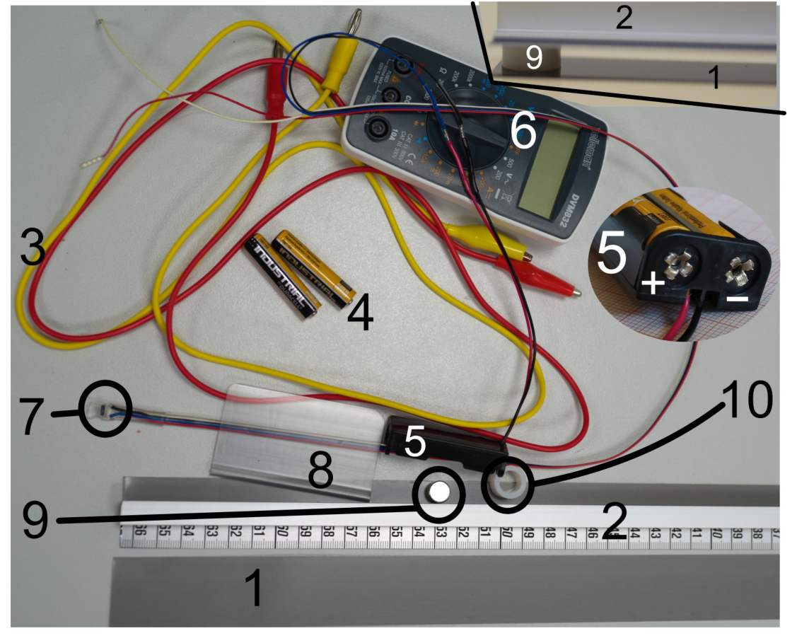
The following equipment is listed in figure 3:

1 — a stand-alone ferromagnetic strip;

2 — a ferromagnetic strip reinforced with an aluminium bar and equipped with a measuring tape;

3 — wires with crocodile clips;

4 — batteries;

5 — a battery holder;

6 — a multimeter;

7 — a resistive magnetic field sensor;

8 — a plastic clamp for fixing the orientation of the sensor;

9 — a magnet;

10 — a plastic spacer to keep the strip (2) strictly horizontal.

Not shown in the figures: a piece of polyethylene film for wrapping the magnet.

WARNINGS:

Do not bend the ferromagnet, as it will become unusable! If bent, no replacement will be provided and you will get no marks for that part.
Avoid direct or reflected laser beams hitting your eye, this can be harmful to your eye!
The syringe needles are sharp, avoid puncturing yourself!
Avoid short-circuiting the battery leads — the battery will overheat and become unusable!
Power off the multimeter and the laser when not in use, in order to conserve the batteries.

Two photos of the diffraction setup. A: laser beam reflected by the mirror (back) towards the screen 1, with clothespin 8 and needle 4 marked, and a zoomed insert of the diffraction pattern on the screen (zoom). B: the syringe standing vertically on its cap, illuminated by the green laser. — Figure 4

Tasks

Part A. Diameter of the syringe needle Determine the diameter of the syringe needles using the following procedure.

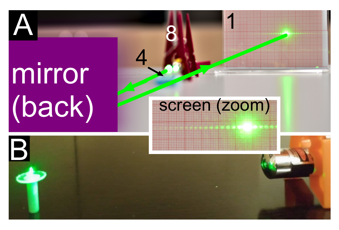
Put the syringe standing vertically onto table, with its plastic cap downside as shown in Fig 4B, install the laser with the help of the clothespins as shown in the figure, and direct the laser beam onto the needle. If the laser beam is too high (i.e. passes the needle above it), you may use the piece of foam as shown in Fig 4A (insert the sharp end of the green syringe needle into the foam so that it will stand vertically). If the laser beam is slightly too low, you may use a folded sheet of paper to raise it. If the laser runs out of battery, you may ask for a replacement. Use the mirror to increase the length of the laser beam (see Fig 4A). Measure the distance between diffraction maxima on the screen as precisely as possible (explain how you achieved the best possible accuracy). Measure the length of the light beam from the syringe needle to the screen and calculate the diameter of the needle. Wavelength of the laser beam is $\lambda = 532\,\mathrm{nm}$ .

Estimate the uncertainty of your result. Repeat the procedure with the white needle. [3 т.]

Part B. Surface tension of water Fill the silicon tube with water — you may use the syringe (do not use the needle!) so that approximately 2/3rd of it is filled with water (adjust the amount of water as needed later); make sure that the water forms a continuous column with no air gaps. Using clamps, fix the tube from its two ends to the screen (which is now used as a stand). Insert the green syringe needle into the tube by puncturing it with the sharp end of the needle. Make sure to puncture the tube perpendicularly near its centre, so that the flat end of the needle will point vertically downwards. Depending on the height of the water column above the open end of the needle, water may or may not start slowly dripping out. If it does not drip, lower the needle by pulling the tube from its middle part downwards so that it will start approaching a V-shape. If water still does not start dripping, add more water into the tube (if even this is not enough, ask for a replacement needle).

While the water is slowly dripping from the needle, raise very slowly the needle to determine, at which height will the dripping stop, and measure the corresponding water column height (the height difference between the water level in the tube, and the lowest point of the needle).

Hint: when the tube is hanging in a U-shaped manner, the height of the water column can be adjusted by pulling the tube from its middle point into a V-shape, or raising it into a W-shape.

Make several measurements with the green needle, and repeat the whole procedure with the white needle. State your results for the critical water column heights together with the uncertainties, for the both needles. Based on your measurements, determine the coefficient of surface tension $\sigma$ for water, alongside its uncertainty. Density of water is $\rho_w = 1000\,\mathrm{kg/m^3}$ , free fall acceleration $g = 9.81\,\mathrm{m/s^2}$ .

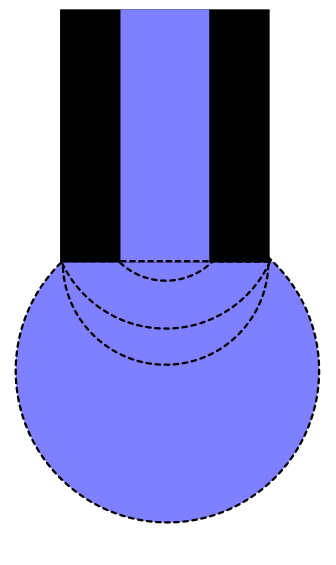
Hints: different stages of the droplet growing from the end of the syringe needle are shown in Fig 5. Surface tension gives rise to a pressure drop over a curved water surface; in the case of a spherical surface, this pressure drop equals to $\Delta p = 2\sigma/r$ , where $r$ is the radius of the spherical surface. [4 т.]

Sketch of the end of a syringe needle (black walls, blue water) with a large spherical water droplet below it; dashed arcs show earlier stages of the droplet growing. — Figure 5

Part C. Susceptibility of graphite Measure the diameter of the magnet and write down the result.

Fill the Petri dish with water so that the water layer depth is approximately half of the dish height. Break a tiny piece from the graphite bar and put it onto the water; it should remain floating owing to surface tension.

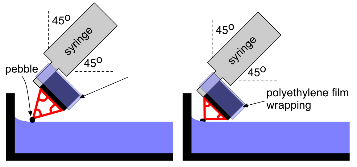
Fix the magnet to the syringe as shown in Fig. 6 (magnet’s axis should be parallel to the syringe) with the help of a piece of the polyethylene film. Orient the magnet approximately under 45 degrees to the horizon (so that the angle between the syringe and vertical direction equals approximately to the angle between the syringe and the horizontal plane). When you move the magnet closer to the piece of graphite, it will “swim” away due to diamagnetism. Push it towards a wall of the Petri dish. When the magnet is not too far away from the wall, for each position of the magnet, there is an equilibrium position of the graphite pebble. You need to achieve two different equilibrium configurations: (a) the magnet’s diameter and the graphite pebble form approximately an equilateral triangle; (b) the magnet’s diameter and the graphite pebble form approximately an isosceles right triangle, see Fig. 6.

Using the ruler, measure the distance between the pebble and the wall of the dish for the both configurations; repeat measurements several time to reduce uncertainty.

The pushing force exerted on the graphite pebble per unit mass of the pebble is given by the formula

\frac{F}{m} = (|\chi_g - \chi_w|)\frac{1}{2\mu_0}\frac{\mathrm{d}B^2}{\mathrm{d}z},

where $\chi_g$ and $\chi_w = -9.05\times 10^{-9}\,\mathrm{m^3/kg}$ are the specific susceptibilities of the graphite and of the water (per unit mass of the material), and $\frac{1}{2\mu_0}\frac{\mathrm{d}B^2}{\mathrm{d}z}$ denotes the magnetic pressure gradient.

Fig. 7 shows the water surface slope angle $\alpha$ as a function of the horizontal displacement $x$ from the vertical wall of the dish, normalized to the characteristic length scale $\sqrt{\sigma/\rho_w g}$ . Here $\rho_w = 1000\,\mathrm{kg}$ is the density of water, and $g = 9.81\,\mathrm{m/s^2}$ is the free fall acceleration. The graphite pebble will rest at very small angles so that the approximation $\alpha \ll 1$ can be used.

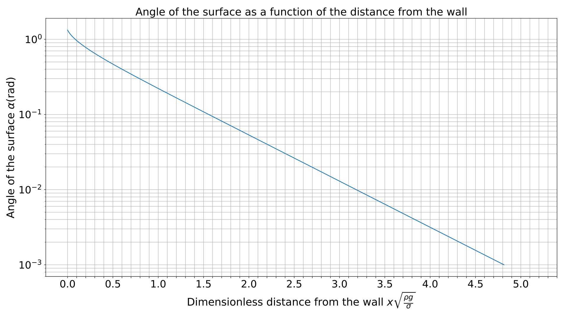
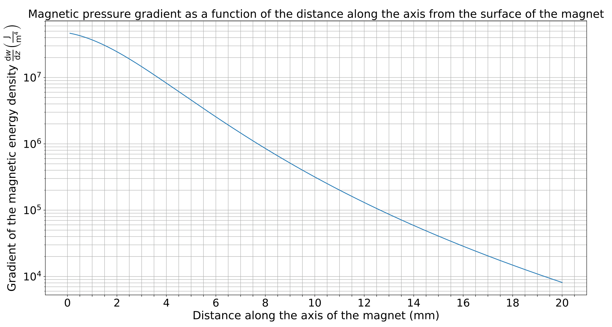
Semi-log graph titled “Angle of the surface as a function of the distance from the wall”: angle of the surface α (rad) from 10^−3 to 10^0 versus dimensionless distance from the wall x√(ρg/σ) from 0 to 5; the curve falls from about 1.3 at 0 to 10^−3 near 4.8. — Figure 7

Fig. 8 shows the magnetic pressure gradient at the magnet’s axis as a function of distance from the flat face of the given permanent magnet.

Semi-log graph titled “Magnetic pressure gradient as a function of the distance along the axis from the surface of the magnet”: gradient of the magnetic energy density dw/dz (J/m⁴) from 10^4 to above 10^7 versus distance along the axis of the magnet from 0 to 20 mm; the curve falls from about 4.5·10^7 at 0 to about 8·10^3 at 20 mm. — Figure 8

Based on these data and your measurements from before, determine $\chi_g$ and estimate its uncertainty. [4 т.]

Part D. Relative permeability of ferromagnetic strip i. (1 pt) Measure the voltage $\mathcal{E}$ on the output leads of the battery holder using the multimeter by connecting multimeter to the leads shown as “+” and “−” in the insert of Fig 3 and switching it to 20 volt (DC) range. If the voltage is below $3.0\,\mathrm{V}$ , you may ask for replacement batteries.

Connect the blue and black wires of the magnetic sensor to the batteries in the battery holder, and the red and white wires to the multimeter. If the plastic clamp is put around the four wires near the sensor as shown if Fig 3, the sensor is kept in such a position that vertical magnetic field will be measured. Switch on the multimeter in 200 millivolt (DC) range, put the sensor onto table far away from the magnet and the ferromagnetic strips, take the reading of the multimeter $V_0$ , and write it down. Subtract this voltage reading from all the subsequent readings (to compensate for the zero offset of the sensor, and for the magnetic field of the Earth).

Two sketches of the Petri dish wall and water surface with a syringe inclined at 45° holding the magnet wrapped in polyethylene film; the pebble floats near the wall; in the left sketch the magnet's diameter and the pebble form an equilateral triangle (red), in the right one an isosceles right triangle. Labels: 45°, syringe, pebble, polyethylene film wrapping. — Figure 6

ii. (4 pts) If the battery voltage were to be exactly $3\,\mathrm{V}$ , each millivolt in the reading would correspond to 10 microteslas of the magnetic field strength. However, the reading is proportional to the battery voltage.

Put the stand-alone ferromagnetic strip onto table; place the magnet and the plastic cylindrical spacer onto it, as close as possible to its endpoints (see the insert of Fig 3), and the reinforced strip onto the whole assembly so that a gap of constant width is formed between the strips. Measure the magnetic field strength $B = B(z)$ between the two strips as a function of distance $z$ from the magnet-less end of the strips. Start with the farthest possible position from the magnet, with $z$ equal to a few millimeters, and use $5\,\mathrm{cm}$ increments. For each distance $z$ , move the sensor between the strips horizontally to find the largest possible reading. Tabulate your direct voltage readings together with the corresponding magnetic field strengths.

Theory predicts that in this configuration, the magnetic field between the strips is

B = B_0\cosh(z/\lambda),

where

\lambda = \sqrt{\mu\delta h/2}

and the hyperbolic cosine is defined as $\cosh x = \frac{1}{2}(\mathrm{e}^x + \mathrm{e}^{-x})$ . Here, $\delta = 0.27\,\mathrm{mm}$ stands for the strip thickness and $h$ — for the width of the gap between the two strips. This can be measured using a ruler. Based on your measurements data, draw an appropriate graph to determine the relative magnetic permeability $\mu$ . Find $\mu$ and estimate the uncertainty of your result.

Hints: the given expression for $B(z)$ fails due to the saturation effect if the magnetic field inside the ferromagnetic strip is too large. Calculators usually do have both cosh-function, as well as its inverse function, denoted as acosh or $\cosh^{-1}$ .

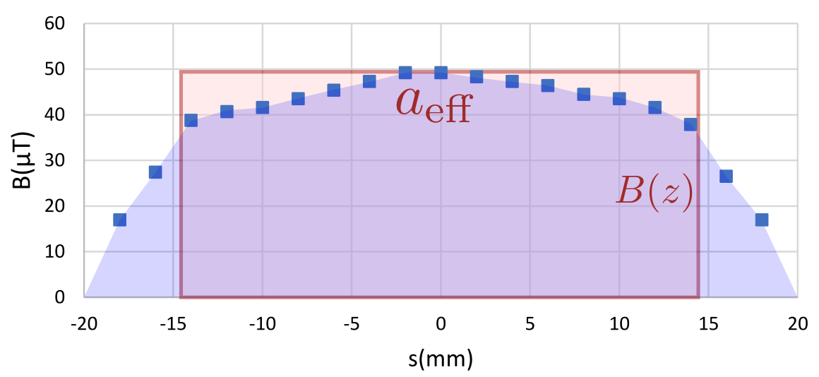
iii. (2 pts) In order to understand how the magnetic flux is distributed over the width of the strip, measure the magnetic field strength as a function of the distance $s$ from the symmetry axis of the strip for a certain fixed value of $z$ in the middle of its range; use $4\,\mathrm{mm}$ -increments and decrease these increments wherever appropriate. Plot the results. Comment on your results.

iv. (2 pts) Assuming that the distribution of the magnetic flux over the width of the strip is almost independent on $z$ , calculate and plot the magnetic field strength inside the ferromagnetic strip as a function of $z$ based on your measurement data (you may take additional measurements if needed). Estimate the field strength $B_s$ by which the magnetization of the ferromagnetic material starts becoming saturated. [9 т.]

Отговори

Решение

Part A. Diameter of the syringe needle (3 points)

In order to maximize the accuracy, the path length of the diffracted laser needs to be maximized since that increases the separation of the maxima on the screen. (0.2 pts) A two-fold increase in the path length can be achieved by using a mirror to reflect the laser from one end of the table to the other and then back again. (0.3 pts)

Sketch of the needle end (black walls, blue water) with a hemispherical water drop below it (dashed outline); an arrow marks the radius r = d/2.

For both needles, the distance from needle to the mirror and from the mirror to the screen were both $L_0 = 119\,\mathrm{cm} \pm 0.5\,\mathrm{cm}$ . The optical path length is then $L = 2L_0 = 238\,\mathrm{cm} \pm 0.5\,\mathrm{cm}$ . (0.3 pts)

On the screen, the optical path difference between two neighbouring maxima is $\lambda$ , which corresponds to a distance of $l_1 = \frac{\lambda}{d}L$ on the screen, where $d$ is the diameter of the syringe needle. In order to increase the accuracy, the measurements should cover as many maxima, $N$ as possible. Then the separation is $l_N = NL\frac{\lambda}{d}$ and $d = \frac{NL\lambda}{l_n}$ . (0.4 pts)

For the white needle, following measurements were made:

$i$	$N$	$l_N$ (mm)	$l_N/N$ (mm)	$d$ (mm)
1	22	89	4.05	0.313
2	18	74	4.11	0.308
3	20	79	3.95	0.321

1 measurement (0.4/0.6 pts)

2 measurements (0.5/0.6 pts)

3 or more measurements (0.6/0.6 pts)

The average diameter is found to be $d = 0.31\,\mathrm{mm}$ (0.1 pts) with an error of $\Delta d = 0.004\,\mathrm{mm}$ . (0.2 pts)

For the green needle, following measurements were made:

$i$	$N$	$l_N$ (mm)	$l_N/N$ (mm)	$d$ (mm)
1	18	98	5.44	0.233
2	15	76	5.07	0.250
3	16	85	5.31	0.238

1 measurement (0.4/0.6 pts)

2 measurements (0.5/0.6 pts)

3 or more measurements (0.6/0.6 pts)

The average diameter is found to be $d = 0.24\,\mathrm{mm}$ (0.1 pts) with an error of $\Delta d = 0.005\,\mathrm{mm}$ . (0.2 pts)

Part B. Surface tension of water (4 points)

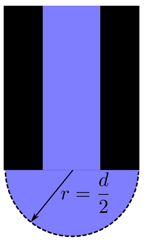
After correctly setting up the equipment and pulling the middle part downwards, the needle should start dripping at one point. This happens because the surface tension isn’t enough to hold back the additional pressure pushing the water down. Note that the critical case is when the radius of curvature of the water drop is the smallest, because then the extra pressure, $2\sigma/r$ , is the biggest. This happens when $r = d/2$ , shown in the figure below. (0.6 pts)

The pressure balance reads

2\sigma/r = \rho g h,

where $\rho g h$ is the pressure from the water column of height $h$ with respect to the needle. If we measure $h$ , we can thus express the surface tension as

\sigma = \frac{\rho g h r}{2} = \frac{\rho g h d}{4}. \qquad (1)

(0.6 pts)

The following repeated measurements were made for the white needle:

$i$	$h$ (mm)
1	84
2	80
3	83
4	82
5	83

1 measurement (0.2/0.6 pts)

2-4 measurements (0.4/0.6 pts)

5 or more measurements (0.6/0.6 pts)

The average height is found to be $h_{\mathrm{avg}} = 82.4\,\mathrm{mm}$ with an error of $\Delta h_{\mathrm{avg}} = 0.7\,\mathrm{mm}$ , and using (1), we get $\sigma = 63.4\,\mathrm{mN/m}$ with an error of $\Delta\sigma = \sigma\sqrt{(\Delta h_{\mathrm{avg}}/h_{\mathrm{avg}})^2 + (\Delta d/d)^2} = 1\,\mathrm{mN/m}$ .

values (0.3 pts)

errors (0.4 pts)

The measurements for the green needle were:

$i$	$h$ (mm)
1	114
2	113
3	116
4	112
5	113

1 measurement (0.2/0.6 pts)

2-4 measurements (0.4/0.6 pts)

5 or more measurements (0.6/0.6 pts)

The average height is $h_{\mathrm{avg}} = 113.6\,\mathrm{mm}$ with an error $\Delta h_{\mathrm{max}} = 0.7\,\mathrm{mm}$ . That gives $\sigma = 67.0\,\mathrm{mN/m}$ , and an error of $\Delta\sigma = 1.5\,\mathrm{mN/m}$ .

values (0.3 pts)

errors (0.4 pts)

The final expression for the surface tension is found by averaging the results of the white and green needle. This yields

$\sigma = (\sigma_{\mathrm{white}} + \sigma_{\mathrm{green}})/2 = 65.2\,\mathrm{mN/m}$ , (0.1 pts)

$\Delta\sigma = \sqrt{\Delta\sigma_{\mathrm{white}}^2/2 + \Delta\sigma_{\mathrm{green}}^2/2} = 1.3\,\mathrm{mN/m}$ . (0.1 pts)

Part C. Susceptibility of graphite (4 points)

Taking only 1 measurement of the diameter of the magnet is enough since the measurement results are all virtually the same. The error of the result comes from the accuracy of a ruler, taken to be $0.3\,\mathrm{mm}$ . The diameter of the magnet is measured to be $d = 10.0\,\mathrm{mm}$ .

value (0.3 pts)

error (0.2 pts)

In both configurations, the graphite will experience three forces: gravity, normal force and magnetic force, all of them being in balance, with the magnetic force being at an angle $45^{\circ}$ with respect to the horizon. Purely under the force of gravity, the graphite would start accelerating with acceleration $a_g \approx g\alpha$ (where we have used small angle approximations) along the water surface (normal force does not contribute to this as it’s perpendicular to the surface). Since the angles are small, this translates to horizontal acceleration of the same magnitude. This is counteracted by the acceleration from the magnet, given by the formula

explaining the force balance (0.5 pts)

a_m = \frac{F}{m} = (|\chi_g - \chi_w|)\frac{1}{2\mu_0}\frac{\mathrm{d}B^2}{\mathrm{d}z} = (|\chi_g - \chi_w|)\frac{\partial w}{\partial z}.

Since the magnet is pushing the graphite at a $45^{\circ}$ angle, the force balance is $a_m/\sqrt{2} = a_g$ . This let us express $\chi_g$ in terms of the measured quantities $\alpha$ and $\frac{\partial w}{\partial z}$ :

\chi_g = \chi_w - \left|\frac{\sqrt{2}g\alpha}{\frac{\partial w}{\partial z}}\right|. \qquad (2)

(0.6 pts)

Here we’ve been careful with the signs, since graphite must have a larger susceptibility in magnitude than water but it’s still negative. This concludes the necessary theoretical calculations.

In the first configuration with the equilateral triangle, following measurements for the distance from the wall were made:

$i$	$l$ (mm)
1	12
2	10
3	11
4	10
5	11

1-2 measurement (0.3/0.5 pts)

3-4 measurements (0.4/0.5 pts)

5 or more measurements (0.5/0.5 pts)

this gives an average of $l = 10.8\,\mathrm{mm}$ with an error of $\Delta l = 0.4\,\mathrm{mm} + 0.5\,\mathrm{mm} = 0.9\,\mathrm{mm}$ , where we have added the measurement error from the ruler and the standard deviation from the tabulated data (we usually omit the ruler’s accuracy in the case of repeat measurements, but that’s usually because the ruler’s accuracy is much smaller than standard deviation).

The corresponding surface slope can be read from the graph, but first we need to convert $l$ to units of $\lambda = \sqrt{\sigma/(\rho g)} = 2.58\,\mathrm{mm}$ , with $\Delta\lambda = 0.03\,\mathrm{mm}$ . Thus, $l = (l/2.58\,\mathrm{mm})\lambda = 4.2\lambda$ with $\Delta l = 0.4\lambda$ . From figure 7, we measure

\alpha = 2.4\times 10^{-3}\,\mathrm{rad}.

\Delta\alpha = 1.8\times 10^{-3}\,\mathrm{rad}

where the error was measured from the figure by looking at $\alpha(\lambda \pm \Delta\lambda)$ . The error is big but this is to be expected due to the exponential nature of the graphs.

To get a reading of the magnetic pressure gradient, we first calculate the distance of the graphite from the surface of the magnet. We see that the distance is that of the height of an equilateral triangle with side length $d = 10\,\mathrm{mm} \pm 0.3\,\mathrm{mm}$ . The distance is then simply $l_1 = \sqrt{3}/2d = 8.7\,\mathrm{mm} \pm 0.3\,\mathrm{mm}$ . From figure 8, we read the magnetic pressure gradient to be $\frac{\partial w}{\partial z} = 6.1\times 10^5\,\mathrm{J/m^4} \pm 0.9\times 10^5\,\mathrm{J/m^4}$ .

Finally, using equation (2), we find

\chi_g = 6.4\times 10^{-8}\,\mathrm{m^3/kg} \pm 4\times 10^{-8}\,\mathrm{m^3/kg}.

reading the data from the graphs properly (0.2 pts)

final value for $\chi_g$ (0.1 pts)

error propagation (0.3 pts)

We go through the same calculations in the 2nd configuration to get a different estimate for $\chi_g$ . The measurements for 2nd configuration are tabulated below

$i$	$l$ (mm)
1	7
2	8
3	8
4	6
5	7

1-2 measurement (0.3/0.5 pts)

3-4 measurements (0.4/0.5 pts)

5 or more measurements (0.5/0.5 pts)

We find $l = 7.2\,\mathrm{mm}$ , $\Delta l = 0.4\,\mathrm{mm} + 0.5\,\mathrm{mm} = 0.9\,\mathrm{mm}$ . This corresponds to $l = 2.8\lambda \pm 0.4\,\lambda$ From figure 7, we read $\alpha = 1.7\times 10^{-2}\,\mathrm{rad} \pm 0.9\times 10^{-2}\,\mathrm{rad}$ .

In this case, a right-angled isosceles is formed. It’s easy to see that the graphite is distance $d/2 = 5\,\mathrm{mm} \pm 0.15\,\mathrm{mm}$ from the surface of the magnet. This gives the magnetic pressure gradient to be $\frac{\partial w}{\partial z} = 4.6\times 10^6\,\mathrm{J/m^4} \pm 0.4\times 10^6\,\mathrm{J/m^4}$ . This gives the susceptibility to be $\chi_g = 6.0\times 10^{-8}\,\mathrm{kg/m^3} \pm 3\,\mathrm{kg/m^3}$ .

reading the data from the graphs properly (0.2 pts)

final value for $\chi_g$ (0.1 pts)

error propagation (0.3 pts)

Finally, we average the two results to get

\chi_g = 6.2\times 10^{-8}\,\mathrm{kg/m^3} \pm 4\times 10^{-8}\,\mathrm{kg/m^3}.

final answer (0.1 pts)

error (0.1 pts)

Part D. Relative permeability of ferromagnetic strip (9 points)

i. (1 pt) The voltage on the output leads of the battery holder can be measured to be $\mathcal{E} = 3.17\,\mathrm{V}$ , no uncertainty is needed. (0.5 pts)

After correctly setting up the experimental equipment, the zero off-set is measured to be $V_0 = 2\,\mathrm{mV}$ . (0.5 pts)

ii. (4 pts) Rearranging the expression for the magnetic field strength between the strips, $B = B_0\cosh(z/\lambda)$ , we get

\cosh^{-1}(B/B_0) = z/\lambda. \qquad \textbf{(0.5 pts)}

We can measure $z$ and $V$ , and $V$ can be converted into magnetic field strength $B$ by noting that the maximal field strength $B_{\max} = 3\,\mathrm{V}\cdot\frac{10\,\mathrm{\mu T}}{1\,\mathrm{mV}} = 30\,\mathrm{mT}$ is measured at $V = \mathcal{E}$ , and thus, we must have

B = B_{\max}\frac{V}{\mathcal{E}} = 30\,\mathrm{mT}\cdot\frac{V}{\mathcal{E}}. \qquad (3)

(0.3 pts)

This relies on the fact that the magnetic field strength scales linearly with voltage. To linearize the measured data, we need to know $B_0$ . This can be found by noting that $\cosh(0) = 1$ and so $B_0 = B(z = 0)$ . This we can read from the measured data to be $B_0 = 0.227\,\mathrm{T}$ . (0.2 pts)

Now note that we can plot $\cosh^{-1}(B/B_0)$ against $z$ to get a linear graph with slope $1/\lambda$ . The tabulated data is given below.

$z$ (cm)	$V$ (mV)	$B$ (mT)	$\cosh^{-1}(B/B_0)$
0	24	0.227	0.130
5	25	0.237	0.316
10	27	0.256	0.513
15	30	0.284	0.707
20	35	0.331	0.936
25	44	0.416	1.225
30	52	0.492	1.418
35	58	0.549	1.539
40	71	0.672	1.757
45	85	0.804	1.946
50	104	0.984	2.154
55	200	1.893	2.818

less than 3 measurements (0.0/0.4 pts)

3 - 11 measurements (0.2/0.4 pts)

correct number of measurements (0.4/0.4 pts)

calculations (0.4 pts)

It is important to note that on the graph, the line doesn’t need to pass through origin due to systematic errors affecting all the points equally. For example, the measured $z = 0$ doesn’t coincide with the actual origin due to the physical dimensions of the magnet. Furthermore, the final point in the graph is not used for fitting since it deviates due to the over saturation effect.

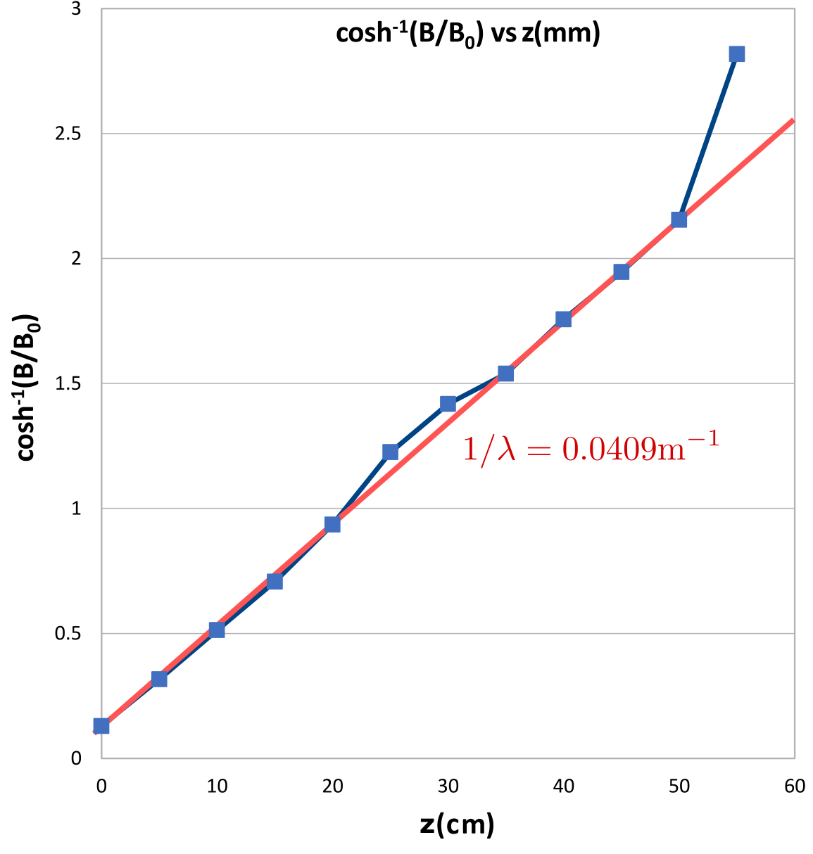
Graph titled “cosh⁻¹(B/B0) vs z(mm)”: cosh⁻¹(B/B0) from 0 to 3 versus z(cm) from 0 to 60; blue data points joined by a line and a red fitted straight line labelled 1/λ = 0.0409 m⁻¹; the last point at z = 55 lies well above the line.

plotting (1.0 pts)

From the graph, we read the slope to be $1/\lambda = 0.0409\,\mathrm{m^{-1}}$ .

(0.2 pts)

The uncertainty can be estimated by looking at the spread of lines that can be reasonably expected to pass through the points. This yields $\Delta(1/\lambda) = 0.000\,72\,\mathrm{m^{-1}}$ . (0.2 pts)

Now, $\mu = \frac{2\lambda^2}{\delta h}$ . We measure $h$ , the width of the gap, with a ruler to be $h = 7.7\,\mathrm{mm} \pm 0.3\,\mathrm{mm}$ . The error is found by noting that the error of a ruler is half, or slightly less depending on how good your eye is, of the distance between two neighbouring ticks, $0.1\,\mathrm{mm}$ . Finally, we calculate $\mu = 57\,000$ (0.4 pts) with an error of

\Delta\mu = \mu\sqrt{\left(2\frac{\Delta(1/\lambda)}{(1/\lambda)}\right)^2 + \left(\frac{\Delta h}{h}\right)^2} = 3000. \qquad \textbf{(0.4 pts)}

iii. (2 pts) The tabulated measurement data is given below. The voltages are translated to teslas using equation (3).

$x$ (mm)	$s$ (mm)	$V$ (mV)	$B$ (mT)
0	-18	18	0.170
2	-16	29	0.274
4	-14	41	0.388
6	-12	43	0.407
8	-10	44	0.416
10	-8	46	0.435
12	-6	48	0.454
14	-4	50	0.473
16	-2	52	0.492
18	0	52	0.492
20	2	51	0.483
22	4	50	0.473
24	6	49	0.464
26	8	47	0.445
28	10	46	0.435
30	12	44	0.416
32	14	40	0.379
34	16	28	0.265
36	18	18	0.170

less than 3 measurements (0.1/0.6 pts)

3 - 5 measurements (0.3/0.6 pts)

6 - 7 measurements (0.4/0.6 pts)

correct number of measurements (0.6/0.6 pts)

calculations (0.4 pts)

$x$ is measured with respect to the first data point, $s$ is with respect to the symmetry axis (found to be at $x = 18\,\mathrm{mm}$ ). The graph for $B$ vs $s$ is given below.

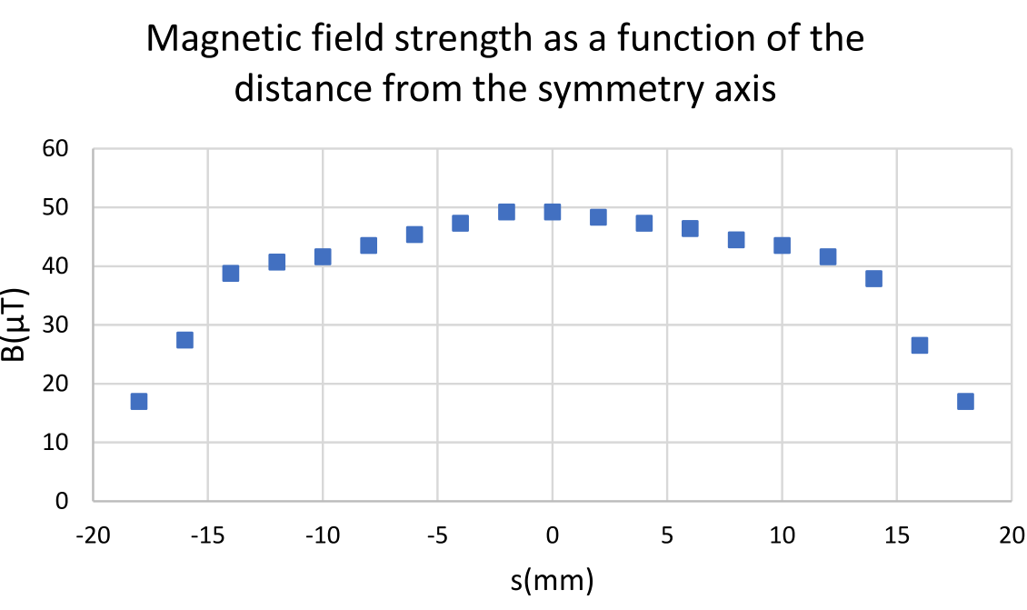
Scatter plot titled “Magnetic field strength as a function of the distance from the symmetry axis”: B(µT) from 0 to 60 versus s(mm) from −20 to 20; the points form a plateau near 40–50 and drop to about 17 at s = ±18.

plotting (0.6 pts)

As can be seen, the magnetic field strength is uniform and with small deviations up to $\sim 10\,\%$ over the width of the strip. Outside the strip, the field strength starts dropping rapidly. (0.4 pts)

iv. (2 pts) The main idea relies on the fact that magnetic field lines are conserved, or in other words the magnetic flux through a closed surface is 0. This is equivalent to Gauss’ law. In the context of this problem, it implies that the flux entering the gap must come from the decrease of the flux flowing along the ferromagnetic strip. The flux flowing outside the strip will be negligible because of the high value of $\mu$ .

Let the total flux along the strip be $\Phi_{\mathrm{in}}$ , $z$ -axis be along the strip, and $x$ -axis be horizontal, perpendicular to $z$ . Also denote the flux through the $x - z$ plane intersecting the gap from $z = 0$ to $z$ as $\Phi_z$ . The Gauss’ law can then be formulated as

\Phi_{\mathrm{in}}(z) - \Phi_{\mathrm{in}}(z = 0) = \Phi_z. \qquad (4)

(0.5 pts)

Note that since the flux inside the ferromagnet drops exponentially, and judging from the tabulated data, it’s reasonable to say that $\Phi_{\mathrm{in}}(z) \gg \Phi_{\mathrm{in}}(z = 0)$ . (0.1 pts) We can approximate the magnetic field to be homogeneous throughout the cross-section of the ferromagnet (to very high accuracy, this can be verified using Ampère’s law). Then $\Phi_{\mathrm{in}}(z) = a\delta B_{\mathrm{in}}(z)$ , where $a$ is the width of the ferromagnet, measured to be $a = 30\,\mathrm{mm} \pm 0.3\,\mathrm{mm}$ , and $B_{\mathrm{in}}(z)$ is the magnetic field inside the ferromagnet. (0.1 pts)

This means that if we calculate $\Phi_z$ , we can find $B_{\mathrm{in}}$ using equation (4). To find $\Phi_z$ , we need to sum the magnetic field over the $z$ - and $x$ -direction. In integral form, it looks like $\Phi_z = \int_0^z \mathrm{d}z' \int_{-\infty}^{\infty} \mathrm{d}x B(x, z')$ . We can simplify this with the integral $\Phi_z = a_{\mathrm{eff}}\int_0^z \mathrm{d}z' B(z')$ , where $a_{\mathrm{eff}}$ is the effective width of the gap such that the area under the graph found in the previous part is equal to $B(z')a_{\mathrm{eff}}$ , where $B(z')$ is the maximal magnetic field in the gap found in part (ii).

Graph titled “Magnetic field strength inside the strip as a function of z”: B_in(T) from 0 to 1.2 versus z(cm) from 0 to 60; points joined by a rising curve from 0.04 at z = 5 to about 1.08 at z = 55.

From an approximate plot shown below, we find $a_{\mathrm{eff}} = 0.955a = 28.7\,\mathrm{mm}$ .

The B(µT) versus s(mm) scatter plot with a shaded area under the data and a red rectangle of height B(z) and width a_eff of equal area, labelled a_eff and B(z).

Finding $a_{\mathrm{eff}}$ using a plot, or something equivalent (0.2 pts)

All that’s left is to find $\int_0^z \mathrm{d}z' B(z')$ . This can be found from the tabulated data found in part (ii) by summing over the data points using the trapezoid rule,

\begin{aligned} \Phi_i &= \Phi_{i-1} + \frac{B_i + B_{i-1}}{2}(z_i - z_{i-1})a_{\mathrm{eff}} \\ &= \Phi_{i-1} + \frac{B_i + B_{i-1}}{2}\Delta A = \Phi_{i-1} + \Delta\Phi_i, \end{aligned}

(0.3 pts)

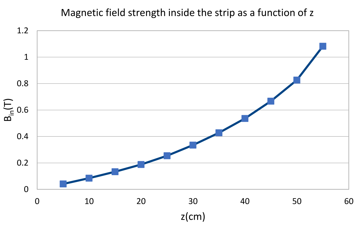
where $\Delta A = (z_i - z_{i-1})a_{\mathrm{eff}} = 5\,\mathrm{cm}\cdot 28.7\,\mathrm{mm} = 0.001\,44\,\mathrm{m^2}$ is the effective area of the last segment and $\Delta\Phi_i = \frac{B_i + B_{i-1}}{2}\Delta A$ the flux through the corresponding surface. After that, the magnetic field inside the ferromagnetic is simply found using (4) as $B_{\mathrm{in}} = \frac{\Phi_{\mathrm{in}}}{a\delta}$ .

The calculated data is given below alongside with the plot of $B_{\mathrm{in}}$ vs $z$ .

$z$ (cm)	$B$ (mT)	$\Delta\Phi$ ( $\mathrm{\mu T\cdot m^2}$ )	$\Phi$ ( $\mathrm{\mu T\cdot m^2}$ )	$B_{\mathrm{in}}$ (T)
0	-	-	0
5	0.232	0.334	0.334	0.041
10	0.246	0.354	0.688	0.085
15	0.27	0.389	1.077	0.133
20	0.308	0.444	1.521	0.188
25	0.374	0.539	2.06	0.254
30	0.454	0.654	2.714	0.335
35	0.521	0.75	3.464	0.428
40	0.61	0.878	4.342	0.536
45	0.738	1.063	5.405	0.667
50	0.894	1.287	6.692	0.826
55	1.438	2.071	8.763	1.082

calculations (0.3 pts)

plotting (0.3 pts)

Since in the graph found in part (ii), the saturation cut-off happened at the last data point, we can use the corresponding value for $B_{\mathrm{in}}$ as an estimate for $B_s$ . Then $B_s \sim 1.1\,\mathrm{T}$ . (0.2 pts)

Оригинал в Архива: exp.pdf · официални решения: exp_sol.pdf