Съдържание

Условие 2.1.2.2.2.3.Summary Answer Sheet — (D2) Compact Object in a Binary System Решение

IOAA 2018, Анализ на данни — D2. Compact Object in a Binary System

Оригинал на условието (PDF)Съобщи за грешка

Всички материали от IOAA 2018

12th International Olympiad on Astronomy and Astrophysics — Data Analysis Competition · 75 т.

Указания

The data analysis competition lasts for 5 hours and is worth a total of 150 points.
Dedicated IOAA Summary Answer Sheets are provided for writing your answers. Enter the final

answers into the appropriate boxes in the corresponding Summary Answer Sheet. On each Answer
Sheet, please fill in

Student’s Code

Graph Paper is required for your solutions. On each Graph Paper sheet, please fill in
- Student’s Code
- Question no.
- Graph no. and total number of graph paper sheets used.
There are Answer Sheets for carrying out detailed work/rough work. On each Answer Sheet, please

fill in

Student’s Code
Question no.
Page no. and total number of pages.

Start each problem on a separate Answer Sheet. Please write only on the printed side of the sheet.

Do not use the reverse side. If you have written something on any sheet which you do not want to be marked, cross it out.

Use as many mathematical expressions as you think may help the graders to better understand your

solutions. The graders may not understand your language. If it is necessary to explain something in words, please use short phrases (if possible in English).

You are not allowed to leave your working desk without permission. If you need any assistance

(malfunctioning calculator, need to visit a restroom, need more Answer Sheets, Graph Paper etc.), please put up your hand to signal the invigilator.

The beginning and end of the competition will be indicated by a long sound signal. Additionally,

there will be a short sound signal fifteen minutes before the end of the competition (before the final long sound signal).

At the end of the competition you must stop writing immediately. Sort and put your Summary

Answer Sheets, Graph Papers, and Answer Sheets in one stack. Put all other papers in another stack.
You are not allowed to take any sheet of paper out of the examination area.

Wait at your table until your envelope is collected. Once all envelopes are collected, your student

guide will escort you out of the competition room.

A list of constants is given on the next page.

Table of constants

Group	Quantity	Value
Earth	Mass	$5.98\times10^{24}\ \mathrm{kg}$
Earth	Radius	$6.38\times10^6\ \mathrm{m}$
Earth	Acceleration of gravity	$9.81\ \mathrm{m\,s^{-2}}$
Earth	Obliquity of Ecliptic	23°27′
Earth	Length of Tropical Year	365.2422 mean solar days
Earth	Length of Sidereal Year	365.2564 mean solar days
Earth	Albedo	0.39
Moon	Mass	$7.35\times10^{22}\ \mathrm{kg}$
Moon	Radius	$1.74\times10^6\ \mathrm{m}$
Moon	Mean Earth-Moon distance	$3.84\times10^8\ \mathrm{m}$
Moon	Orbital inclination with the Ecliptic	5.14°
Moon	Albedo	0.14
Moon	Apparent magnitude (mean full moon)	−12.74
Sun	Mass	$1.99\times10^{30}\ \mathrm{kg}$
Sun	Radius	$6.96\times10^8\ \mathrm{m}$
Sun	Luminosity	$3.83\times10^{26}\ \mathrm{W}$
Sun	Absolute Magnitude	4.80 mag
Sun	Surface Temperature	5772 K
Sun	Angular diameter at Earth	30′
Sun	Orbital velocity in Galaxy	$220\ \mathrm{km\,s^{-1}}$
Sun	Distance from Galactic center	8.5 kpc
Physical constants	1 au	$1.50\times10^{11}\ \mathrm{m}$
Physical constants	1 pc	206265 au
Physical constants	Gravitational constant (G)	$6.67\times10^{-11}\ \mathrm{N\,m^2\,kg^{-2}}$
Physical constants	Planck constant (h)	$6.62\times10^{-34}\ \mathrm{J\,s}$
Physical constants	Boltzmann constant	$1.38\times10^{-23}\ \mathrm{J\,K^{-1}}$
Physical constants	Stefan-Boltzmann constant	$5.67\times10^{-8}\ \mathrm{W\,m^{-2}\,K^{-4}}$
Physical constants	Hubble constant	$67.8\ \mathrm{km\,s^{-1}\,Mpc^{-1}}$
Physical constants	Speed of light in vacuum	299792458 m/s
Physical constants	Magnetic Permeability of free space	$4\pi\times10^{-7}\ \mathrm{H\,m^{-1}}$
Physical constants	1 Jansky (Jy)	$10^{-26}\ \mathrm{W\,m^{-2}\,Hz^{-1}}$

\Delta\log_{10}(x)=\frac{\Delta x}{x\ln10}.

Бележки за изданието

The independently archived question and solution PDFs are the source editions used here. D1.4 remains in the questions, answer form and worked key, but the key explicitly marks its 12 marks “discarded”; printed totals of 75 per problem and 150 overall are retained. Section 1.3 calls $F_{1600}$ “unattenuated” although section 1.2 defines it as observed; the source wording is preserved. The answer form labels the mass-function field D2.2.2 and omits a separate orbital-radius field. D2.3.3 calls the $\sin i+\Delta\sin i$ curve an upper limit and the $\sin i-\Delta\sin i$ curve a lower limit; the official figure places them in the opposite vertical order, as the mass function requires. In the key, equation (19) prints a strict inequality at the radius bound, equation (32) leaves the cgs-to-SI conversion implicit, and the D2.3.4 rubric assigns only four of its printed five marks. These source inconsistencies have not been silently corrected.

The solution PDF repeats an older wording of the questions: $B$ replaces $Q$ , $f(\beta)$ replaces $S(\beta)$ , D1.1.3 explicitly requests least-squares fitting, Table 1 is called UV photometry, and the dex explanation is written $\mathrm{dex}(x)=10^x$ . It additionally gives the 21 µJy ALMA limit and explicit redshift-factor hint reproduced with D1.4. Its APOGEE velocities are rounded to 34.85 and 42.57 km/s; its D2.3.2 options are (1) Blue Giant (2) Blue Dwarf (3) Red Giant (4) Red Dwarf (5) Main-Sequence Star (6) White Dwarf. The question edition’s data and five options are retained above; the official answer remains (3) Red Giant.

Условие

Astronomers discovered an extraordinary binary system in the constellation of Auriga during the course of the Apache Point Observatory Galactic Evolution Experiment (APOGEE). In these questions, you will try to analyse the data and recreate their discovery for yourself.

The research team is aiming to find compact stars in binary systems using the radial velocity (RV) technique. They examined archival APOGEE spectra of “single” stars and measured the apparent variation of their RV within this data. Among ~200 stars with the highest accelerations, researchers searched for periodic photometric variations in data from the All-Sky Automated Survey for Supernovae (ASAS-SN) that might be indicative of transits, ellipsoidal variations or starspots. After this process, they spotted a star named 2M05215658+4359220, with a large variation in RV and photometric variability.

2.1.

The following table presents the radial velocity measurements of 2M05215658+4359220 during three epochs of APOGEE spectroscopic observation. Here we assume the variation of its RV is due to the existence of an unseen companion. The proper motion of the stars can be ignored.

Table 3. APOGEE Radial Velocity Measurements of 2M05215658+4359220

Observation	MJD	RV ( $\mathrm{km\,s^{-1}}$ )	Uncertainty ( $\mathrm{km\,s^{-1}}$ )
1	56204.9537	-37.417	0.011
2	56229.9213	34.846	0.010
3	56233.8732	42.567	0.010

(D2.1.1) Use the data and a simple linear model to obtain an initial estimate of the apparent maximum acceleration of the star:

a_{\max}=\left.\frac{\Delta\mathrm{RV}}{\Delta t}\right|_{\max},\qquad\text{unit: }\mathrm{km\,s^{-1}\,day^{-1}}.

[6 т.]

(D2.1.2) Now use the data to obtain an initial estimate of the mass of its unseen companion. [9 т.]

2.2.

After discovering this peculiar star, astronomers conducted follow-up observations using the 1.5-m Tillinghast Reflector Echelle Spectrograph (TRES) at the Fred Lawrence Whipple Observatory (FLWO) located on Mt. Hopkins in Arizona, USA. The following table presents the RV measurements using this instrument:

Table 4. TRES Radial Velocity Measurements of 2M05215658+4359220

MJD	RV (km/s)	Uncertainty (km/s)
58006.9760	0	0.075
58023.9823	-43.313	0.075
58039.9004	-27.963	0.045
58051.9851	10.928	0.118
58070.9964	43.782	0.075
58099.8073	-30.033	0.054
58106.9178	-42.872	0.135
58112.8188	-44.863	0.088
58123.7971	-25.810	0.115
58136.6004	15.691	0.146
58143.7844	34.281	0.087

(D2.2.1) Plot the diagram of RV variation (measured with TRES) versus time on your graph paper and label it as Figure 4. Draw a suitable sinusoidal function to fit the given data. Estimate the orbital period ( $P_{\mathrm{orb}}$ ) and radial velocity semi-amplitude ( $K$ ) from your plot. [14 т.]

(D2.2.2) If the star is moving in a circular orbit, calculate the minimum value of the orbital radius ( $r_{\mathrm{orb}}$ ) of the star in units of both $R_\odot$ and au. [4 т.]

(D2.2.3) The mass function of a binary system is defined as:

f(M_1,M_2)=\frac{(M_2\sin i_{\mathrm{orb}})^3}{(M_1+M_2)^2}

where the subscript “1” represents the primary star and “2” represents its companion. The parameter $i_{\mathrm{orb}}$ is the orbital inclination of the binary system. This mass function can also be expressed in terms of observable parameters. Calculate the mass function of this system in units of $M_\odot$ . [7 т.]

2.3.

Based on a detailed analysis on APOGEE, TRES spectra and GAIA parallax measurements, astronomers derived the following stellar parameters:

Table 5. Selected Physical Properties of 2M05215658+4359220

Effective Temperature $T_{\mathrm{eff}}$ (K)	Surface Gravity $\log g$ ( $\mathrm{cm\,s^{-2}}$ )	Parallax $\pi$ (mas)	Measured Rotation Velocity $v_{\mathrm{rot}}\sin i$ ( $\mathrm{km\,s^{-1}}$ )	Bolometric Flux $F$ ( $\mathrm{J\,s^{-1}\,m^{-2}}$ )
4890 ± 130	2.2 ± 0.1	0.272 ± 0.049	14.1 ± 0.6	$(1.1\pm0.1)\times10^{-12}$

Photometric observations indicate that the period of its light curve is identical to its orbital period, thus we may assume that the rotation period satisfies $P_{\mathrm{rot}}=P_{\mathrm{orb}}\equiv P$ , and the inclination satisfies $i_{\mathrm{orb}}=i_{\mathrm{rot}}\equiv i$ .

(D2.3.1) Calculate the luminosity ( $L_1$ , in unit of $L_\odot$ ), radius ( $R_1$ , in unit of $R_\odot$ ), sine of the inclination angle ( $\sin i$ ), as well as mass ( $M_1$ , in unit of $M_\odot$ ) of the visible star. Please include the uncertainty in your results. [16 т.]

(D2.3.2) Choose the correct type of this star from the following options: (1) Blue Giant (2) Yellow main sequence star (3) Red Giant (4) Red main sequence star (5) White Dwarf. [4 т.]

(D2.3.3) Based on the mass function $f(M_1,M_2)$ of the binary system, plot the rough relationship of $M_2$ (as vertical axis) and $M_1$ (as horizontal axis) on your graph paper and label it as Figure 5. Plot the most probable relation (by using $\sin i$ ), upper limit (with $\sin i+\Delta\sin i$ ) and lower limit (with $\sin i-\Delta\sin i$ ) derived in (D2.3.1). [10 т.]

(D2.3.4) Draw a vertical shadowed region of $[M_1-\Delta M_1,M_1+\Delta M_1]$ , as well as two horizontal dashed lines showing the maximum mass of the white dwarf and neutron star, on your Figure 5. What is the possible mass of the invisible companion, and what kind of celestial object could it be? [5 т.]

Summary Answer Sheet — (D2) Compact Object in a Binary System

Student’s Code: □□□–□□

(D2.1.1) The maximum acceleration is □ km/s/day;

(D2.1.2) Estimate for the mass of the companion: □ $M_\odot$ ;

(D2.2.1) See Figure 4; $P_{\mathrm{orb}}=$ □; $K=$ □;

(D2.2.2) $f(M_1,M_2)=$ □ $M_\odot$ ;

(D2.3.1) $\sin i=$ □; $R_1=$ □ $R_\odot$ ; $L_1=$ □ $L_\odot$ ; $M_1=$ □ $M_\odot$ ;

(D2.3.2) The type of this star should be □;

(D2.3.3) See Figure 5;

(D2.3.4) The possible mass of the unseen companion is □ $M_\odot$ ; It could be a □.

Решение

Official solution and grading. The repeated questions in the solution PDF use slightly different wording, rounded APOGEE velocities and six stellar-type options; the independently archived question edition above is retained.

2.1. APOGEE RV Measurements [15 marks]

(D2.1.1) Table 3 gives 3 epochs of RV measurements from MJD 56204 to 56233, and the maximum acceleration occurred during the first and the second observation:

a_{\max}=\frac{\mathrm{RV}_2-\mathrm{RV}_1}{t_2-t_1}=2.89\ \mathrm{km/(s\cdot d)}\qquad (15)

[6 т.]

(D2.1.2) An easy approach to estimate the companion mass is consider the force exerted on the star:

F=M_1a=\frac{GM_1M_2}{r^2}\Rightarrow M_2=\frac{ar^2}{G}\qquad (16)

Therefore, we need to estimate $a$ and $r$ properly. Here we can assume the acceleration of the primary star as $a=a_{\max}$ , and the distance between the two star $r=(v_2-v_1)\cdot(t_2-t_1)/2$ , and we can derive:

M_2\sim\frac{(v_2-v_1)^3(t_2-t_1)}{4G}=1.5\ M_\odot\qquad (17)

(Note: This is only a rough estimate. If examinees derive a $M_2$ within the range of $0.5M_\odot\sim3M_\odot$ [4 marks] with clear and proper assumption [5 marks], then his/her solution should be considered correct.) [9 т.]

2.2. TRES RV Measurements [25 marks]

(D2.2.1) Given the data in Table 4, we can plot out all the TRES RV measurements, with a sinusoidal function connecting all the points:

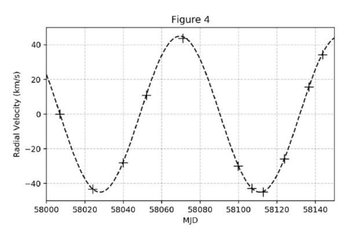
Figure 4. Official TRES radial-velocity sinusoid.

Grading standard of Figure 4: (1) [1 mark] The figure is large enough on the graph paper (larger than 50% of usable space); (2) [2 marks] horizontal axis is MJD, vertical axis is RV (in unit of km/s), and both axes are plotted in linear scale; (3) [1 mark] Ticks on both axes are properly labeled with suitable spacing; (4) [6 marks] Data points and sinusoidal function are plotted properly.

The best-fit parameters of period an RV semi-amplitude are:

P_{\mathrm{orb}}=83.26\pm0.02\ \mathrm d;\quad K=45.02\pm0.03\ \mathrm{km/s}\qquad (18)

(error bars are reported here for benefit of jury. They do not carry any points)

[2 marks for each parameter]

Answers within the range of $P_{\mathrm{orb}}\in[81,85]\ \mathrm d$ and $K\in[44,46]\ \mathrm{km/s}$ could be considered correct. [14 т.]

(D2.2.2) The orbital radius satisfies that:

2\pi R_{\mathrm{orb}}=P_{\mathrm{orb}}\cdot\frac{K}{\sin i_{\mathrm{orb}}}\Rightarrow R_{\mathrm{orb}}>\frac{P_{\mathrm{orb}}K}{2\pi}=74\ R_\odot=0.34\ \mathrm{AU}\qquad (19)

[4 т.]

(D2.2.3) The mass function of a binary system is defined as:

f(M_1,M_2)=\frac{M_2^3\sin^3i_{\mathrm{orb}}}{(M_1+M_2)^2}\qquad (20)

This mass function is actually derived from Newton’s law (force balance):

\frac{GM_1M_2}{D^2}=M_1\left(\frac{2\pi}{P}\right)^2R_{\mathrm{orb}}\qquad (21)

And the relation between orbital radius and binary separation ( $D$ ):

R_{\mathrm{orb}}=\frac{M_2}{M_1+M_2}D=\frac{P_{\mathrm{orb}}K}{2\pi\sin i_{\mathrm{orb}}}\qquad (22)

Therefore, Equation 20 could be rewritten as:

f(M_1,M_2)=\frac{M_2^3\sin^3i_{\mathrm{orb}}}{(M_1+M_2)^2}=\frac{K^3P_{\mathrm{orb}}}{2\pi G}\approx0.79\ M_\odot\qquad (23)

[Equation (21), (22): 2 marks respectively; Equation (23) and the result: 3 marks] [7 т.]

2.3. Stellar Parameters [35 marks]

(D2.3.1) The first (and the most direct) thing we could solve from the given parameter table is the distance of this system, which is:

d=\frac1\pi=3.68\ \mathrm{kpc}\qquad (24)

And the uncertainty of $d$ should be:

\frac{\Delta d}{d}=\sqrt{\left(-\frac{\Delta\pi}{\pi}\right)^2}\Rightarrow\Delta d=\frac{\Delta\pi}{\pi}\cdot d=0.66\ \mathrm{kpc}\qquad (25)

Therefore, the luminosity of the star should be:

L_1=4\pi d^2\cdot F=464\ L_\odot\qquad (26)

And the uncertainty is:

\frac{\Delta L_1}{L_1}=\sqrt{\left(\frac{\Delta F}{F}\right)^2+\left(\frac{2\Delta d}{d}\right)^2}\Rightarrow\Delta L_1=173\ L_\odot\qquad (27)

By using Stefan-Boltzmann law, we can calculate the radius of the star:

R_1=\sqrt{\frac{L_1}{\sigma T^4\cdot4\pi}}=30\ R_\odot\qquad (28)

With an uncertainty of:

\begin{aligned}\Delta R_1&=R_1\sqrt{\left(-2\frac{\Delta T}{T}\right)^2+\left(\frac12\frac{\Delta L_1}{L_1}\right)^2}\\&=R_1\sqrt{\left(-2\frac{\Delta T}{T}\right)^2+\left(\frac12\frac{\Delta F}{F}\right)^2+\left(\frac{\Delta d}{d}\right)^2}=6\ R_\odot\end{aligned}\qquad (29)

Combined with the observed rotational velocity, we can calculate the sine of inclination angle:

\sin i=\frac{P\cdot v\sin i}{2\pi R_1}=0.77\qquad (30)

And the uncertainty should be:

\Delta\sin i=\sin i\sqrt{\left(-\frac{\Delta R_1}{R_1}\right)^2+\left(\frac{\Delta(v\sin i)}{v\sin i}\right)^2}=0.15\qquad (31)

Now we can calculate the mass $M_1$ . First of all, we need to translate the surface gravity from log scale to linear scale:

g=10^{\log g}=1.58\ \mathrm{m/s^2}\qquad (32)

With an uncertainty of:

\Delta g=g\ln10\cdot\Delta(\log g)=0.36\ \mathrm{m/s^2}\qquad (33)

Therefore, $M_1$ should be:

M_1=\frac{gR_1^2}{G}=5.2\ M_\odot\qquad (34)

And the uncertainty is:

\Delta M_1=M_1\sqrt{\left(\frac{\Delta g}{g}\right)^2+\left(2\frac{\Delta R_1}{R_1}\right)^2}=2.3\ M_\odot\qquad (35)

[For each quantity ( $\sin i$ , $R_1$ , $M_1$ , $L_1$ ): deduction: 2 marks; exact value: 1 mark; uncertainty: 1 mark] [16 т.]

(D2.3.2) From the temperature and the luminosity, we can find that the primary star should be a (3) Red Giant. [4 т.]

(D2.3.3) Since we have derived the binary system mass function, with a given range of $M_1$ , we can calculate the corresponding range of $M_2$ and hence make a plot of $M_2-M_1$ (Figure 5). Detailed standards of grading the plot are in the solution of (D2.3.4). [10 т.]

(D2.3.4) The vertical shadowed zone should start at $2.9M_\odot$ and end at $7.5M_\odot$ , while the maximum mass of white dwarf is $1.4M_\odot$ and the maximum mass of neutron star should be around $2.4\sim2.6M_\odot$ (here we adopt $2.5M_\odot$ on the plot). From Figure 5, we can readout that the possible mass of the companion is roughly $6_{-2.5}^{+4}M_\odot$ . Since we didn’t receive any optical radiation from the companion, as well as $M_2$ has already exceeded the maximum mass of neutron star, the invisible companion in this binary system could be a stellar-mass black hole, or some unknown compact object that current theory hasn’t predicted.

[Possible Mass: 2 marks; Type: 2 marks]

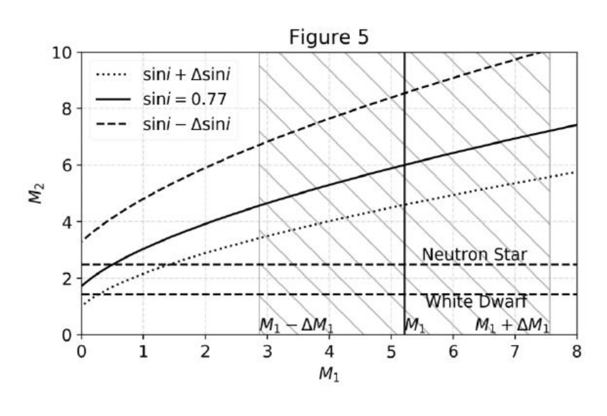
Figure 5. Official mass-function curves, mass range and compact-object limits.

(Note: Examinee’s answer is not required to give an uncertainty range of $M_2$ : if the answer is within the possible range of $6_{-2.5}^{+4}M_\odot$ , the answer will be considered correct. In addition to this, examinee don’t need to include “unknown compact object” in his/her answer while addressing the possible type of the companion: an answer like “black hole” or “stellar-mass black hole” is enough for receiving full grades.)

Grading standard of Figure 5: (1) [1 mark] The figure is large enough on the graph paper (larger than 50% of usable space); (2) [2 marks] horizontal axis is $M_1$ , vertical axis is $M_2$ (both in unit of $M_\odot$ ), and both axes are plotted in linear scale; (3) [1 mark] Ticks on both axes are properly labeled with suitable spacing; (4) [3 mark] All of the three mass functions are plotted properly with obvious and correct labels/legends; (5) [1 mark] Vertical shadowed region of possible $M_1$ range is plotted correctly; (5) [2 marks] Two horizontal dashed lines are plotted at correct positions with clear and correct labels. [5 т.]

Теми и трудност

Трудност: неоценена.

Звезди · Двойни звезди · Компактни обекти

Предпоставки: Разширена олимпиадна подготовка

Оригинал в Архива: Data Analysis Problems.pdf · официални решения: Data Analysis Solutions.pdf · допълнителни данни: 18_da.pdf · допълнителни данни: 18_da_anssheet.pdf · допълнителни данни: 18_da_graph.pdf · допълнителни данни: 18_da_graph_log.pdf