Съдържание

Before the exam During the exam Условие Part 1 (20 т.)Part 2 (16 т.)Part 3 (15 т.)Part 4 (24 т.)Отговори Решение Solar Magnitudes Gauss’s Formulae

IOAA 2021, Анализ на данни — Задача 1. Data Analysis 1: Scaling Relations

Оригинал на условието (PDF)Съобщи за грешка

Всички материали от IOAA 2021

Data Analysis 1: Scaling Relations (75 points) · 75 т.

Внимание: Бележка към темата

The official solution labels 2.1 as 10 points; the question and answer sheet give 6 points, retained in the task scoring. Its references to 1A/1B and positive TF slope in 2.3 are retained as printed. The key mentions a plot on the right in 1.1, but no such plot is printed in the supplied key; all three question graphs are included. The constants sheet prints 23d for a sidereal day and omits solar symbols in several labels; original notation is retained. The three-page blank answer sheet repeats the nine requests and mass table and is included among the original sources.

General instructions: Data Analysis (150 points)

The data analysis competition lasts for 3 hours and is worth a total of 150 points.

Before the exam

You must not open the marked envelopes containing the problems before the signal indicating the beginning of the examination.
The beginning and end of the examination will be marked by a signal from your supervisors, they will also let you know when there are fifteen minutes before the end of the exam.

During the exam

The Data Analysis Examination consists of two parts DA1 and DA2. On your desk you should find a marked envelope with DA1 and DA2. Inside each envelope you will find:
- Cover Sheet for each question with question title, your student code, question code, and your name. Example: Data Analysis 1 (Title) GBR-1 DA-1 John Smith (please make sure these are correct)
- Question Sheets (marked Q)
- Answer Sheets (marked A)
- Working Sheets (marked W)
Dedicated IOAA Answer Sheets (marked A) are provided for writing your answers. Enter the final answers into the appropriate boxes in the corresponding Answer Sheet. Please write only on the printed side of the sheet. Do not use the reverse side. Working Sheets (marked W) are provided for calculations.
Use a black or blue pen for all answers and calculations, this will allow the markers to see your answers better after scanning. If you think you made a mistake cross it out.
Use as many mathematical expressions as you think may help the graders to better understand your solutions. The graders may not understand your language. If it is necessary to explain something in words, please use short phrases (if possible, in English).
You are not allowed to leave your working desk without permission. If you need any assistance (malfunctioning calculator, need to visit a restroom, etc.), please put up your hand to signal the supervisor.
At the end of the competition you must stop writing immediately. Sort your Answer Sheets and Working Sheets for each question (DA1 and DA2) and leave them to be collected in their corresponding envelopes and according to the supervisor's instructions. You are not allowed to take any sheet of paper out of the examination area.

Условие

Please read the general instructions in the separate envelope before you start this problem.

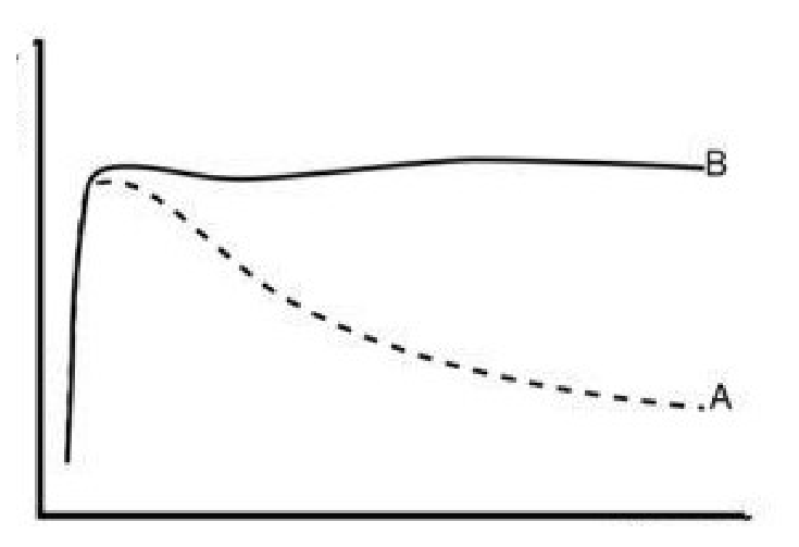
Spiral galaxies are disk-like rotating structures, whose dynamical state is fairly grasped by the so-called rotation curves, quantifying the mean rotational velocity of the disk at different distances from the center (see Figure 1, curve B). An interesting feature is the flat region of the curve, which is attributed to the presence of dark matter. Without it, rotation velocities would drop steadily at large radii from the center, as depicted in curve A.

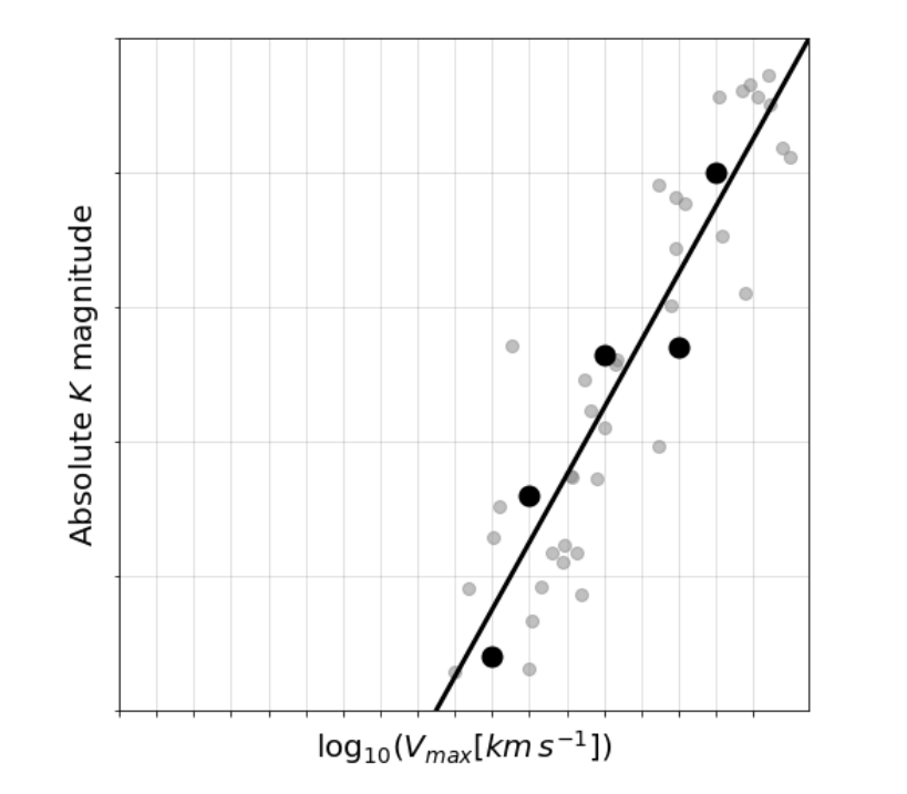
Two rotation curves on unlabelled axes: a solid curve B that rises steeply and then stays flat at large radius, and a dashed curve A that rises to the same peak and then declines steadily with radius. — Figure 1: Rotation curves. Circular velocity (Y-axis) vs Radius (X-axis)

In disk galaxies a strong correlation has been observed between the intrinsic luminosity of the whole galaxy and the asymptotic rotational velocity (as given by the rotation curve for the outer edge of the galaxy i.e. $R_{\mathrm{max}}$ ), a result that is known as the Tully-Fisher relation. This relation also holds if you use the luminosity in a specific band. This is shown on Figure 2 for a number of galaxies in a galaxy cluster. Every dot is a galaxy, and the solid line is the best-fit linear relation between absolute magnitude in $K$ band and $log_{10}(V_{\mathrm{max}})$ for the whole sample.

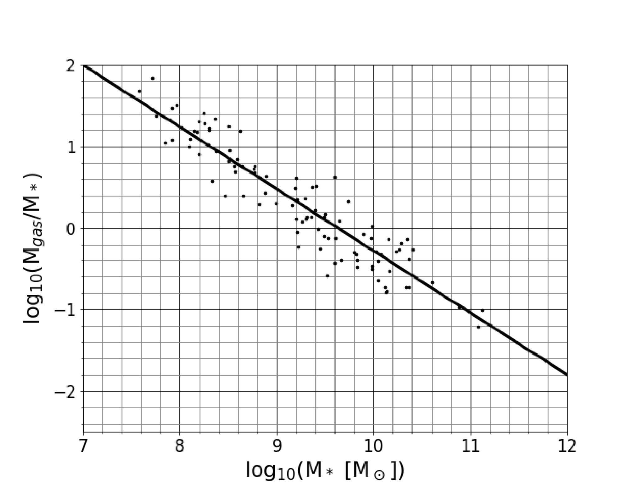
Scatter plot with a grid and no tick values; x-axis labelled log10(Vmax[km s^-1]), y-axis labelled Absolute K magnitude. Grey dots are galaxies, five larger black dots are the selected galaxies, and a solid best-fit straight line runs from lower left to upper right. — Figure 2: Absolute magnitude in $K$ band vs $\log_{10}(V_{\mathrm{max}}[km\,s^{-1}])$ . Tully-Fisher relation for several galaxies. Every dot represents a galaxy. The dark points are five selected galaxies, for which we will provide some numbers in part 1.2.

Scatter plot on a fine grid of log10(Mgas/M*) (y-axis, from -2 to 2) against log10(M* [M_sun]) (x-axis, from 7 to 12). The dots follow a declining trend and a solid straight line runs from (7, 2) down to about (12, -1.8). — Figure 3: Gas fraction vs stellar mass.

Another interesting trend is shown in Figure 3: disks with larger stellar masses ( $M_*$ ) tend to have smaller gas fractions ( $M_{gas}/M_*$ ).

In the following questions you will be asked to extract physical information about the galaxies using the scaling relations just introduced. Consider the following guidelines:

Assume that $V_{\mathrm{max}}$ was measured at the same radius for all galaxies ( $R_{\mathrm{max}}$ ), in the flat part of the rotation curves and well beyond the end of the stellar disk.
Use $M_{dm}$ for the dark matter mass up to $R_{max}$ and $M_{tot}$ for the sum of all components.(gas, stars and dark matter)
Assume that all galaxies have identical stellar populations $^1$ , and assume that the gaseous component does not interact with the stellar light.
The galaxy cluster is far away. Its distance is much larger than the cluster size.
In spherically-symmetric mass distributions, to infer the gravitational effect on a particle at distance $r$ from the center, it suffices to consider the total mass enclosed up to that radius $M(\leq r)$ as if it were placed at the very center of the distribution.

$^1$ The term stellar population refers to the type of stars that are present in a galaxy, and the relative amount of each type with respect to the total number of stars.

Part 1 (20 т.)

1.1 From an analysis of Figure 3, find the appropriate constants in the following relation: $M_{gas} = a \times M_*^b$

a = ?

b = ?

[5 т.]

1.2 In the plot of the Tully-Fisher relation there are 5 highlighted points. Data for these 5 galaxies is given in the following table. Use this dataset to find the appropriate constants for TF relation presented below the table, by means of a linear fit using the method of least squares.

Note: Treat $log_{10}(V_{\mathrm{max}})$ as the $x$ variable and $K$ as the $y$ variable in the linear fit.

$V_{\mathrm{max}}[km/s]$	$K[mag]$
$79.4$	$-16.8$
$100.1$	$-19.2$
$158.5$	$-21.3$
$251.2$	$-21.4$
$316.2$	$-24.0$

K = c \times log_{10}(V_{max}) + d

c = ?

d = ?

[15 т.]

Part 2 (16 т.)

For two galaxies, G1 and G2, in the cluster, the recorded $apparent$ magnitudes are:

k_1 = 19.2 \qquad ; \qquad k_2 = 25.2

Using this information and the relations calibrated in Part 1 find the correct exponents in the following equations:

2.1

\frac{M_{*1}}{M_{*2}} = 10^e \qquad ; \qquad e = ?

[6 т.]

2.2

\frac{M_{gas1}}{M_{gas2}} = 10^f \qquad ; \qquad f = ?

[4 т.]

2.3

\frac{M_{tot1}}{M_{tot2}} = 10^g \qquad ; \qquad g = ?

[6 т.]

Part 3 (15 т.)

3.1

Galaxy	Apparent magnitude $k$	$M_{gas}[M_{\odot}]$	$M_*\ [M_{\odot}]$	$M_{dm}[M_{\odot}]$	$M_{tot}\ [M_{\odot}]$
$G_1$	$19.2$				$4.39\times10^{11}$

Fill in the missing values in the table using the fact that for galaxy $G_1$ , the dark-to-baryonic mass ratio up to $R_{\mathrm{max}}$ is $6.82$ . [15 т.]

Part 4 (24 т.)

4.1 Consider a systematic uncertainty of $\sigma_{sys} = \pm 0.2$ in each apparent magnitude due to CCD calibration errors. Then $k_1$ must be read as $k_1 = 19.2 \pm 0.2$ , i.e., the only thing we know is that $k_1$ most likely lies in the interval $[19.0, 19.4]$ . The same goes for $k_2$ .
Recalculate the exponent in the scaling relation $\frac{M_{*1}}{M_{*2}} = 10^e$ (found in 2.1), expressing $e$ as an interval estimated by considering the extreme possible variations in $k_1$ and $k_2$ .

e \in [?, ?]

[4 т.]

4.2 Now we consider that there is always a natural spread of the data around any relation. For instance, for a given value of the $K$ magnitude the TF relation gives a single value of $log_{10}(V_{\mathrm{max}})$ , but it would be more realistic to report an interval of plausible values, derived from the natural spread of the data around the mean TF relation. We call this the statistical uncertainty, $\sigma_{stat}$ .
Estimate the statistical uncertainty if $log_{10}(V_{\mathrm{max}})$ is inferred from $K$ using the TF relation from question 1.2. For this, consider for each point the difference between the value of $log_{10}(V_{\mathrm{max}})$ estimated from $K$ using your linear fit and the actual measurement of $log_{10}(V_{\mathrm{max}})$ , and take $\sigma_{stat}$ as two times the root mean square (RMS) of these differences $^{\dagger}$ .

\sigma_{stat} = ?

$^{\dagger}$ The RMS of a set of values is the square root of the arithmetic mean of the squares of those values. [10 т.]

4.3 Recalculate the exponent in the scaling relation $\frac{M_{tot1}}{M_{tot2}} = 10^g$ , expressing $g$ as an interval estimated by considering the extreme possible variations arising from both the systematic and statistical uncertainties:

g \in [?, ?]

[10 т.]

Отговори

Решение

Part 1

1.1 From the plot on the right we can get the equation of the straight line as

y = -0.76\cdot x + 7.32 \qquad \text{[3 points]}

which taking to the power of 10 is equivalent to: $f_g = 10^{7.32} M_*^{-0.76}$ , being $f_g$ the gas fraction. Multiplying by the stellar mass we finally get:

M_{gas} = 10^{7.32} \times M_*^{0.24}

a = 10^7.32 = 2.09 E7 [1 point] ; b = 0.24 [1 point]

No tolerance allowed for these values

1.2 [15 points]

V	LogV	K	Zx	Zy	ZxZy
79.4	1.8998	-16.8	-1.1778	1.3873	-1.6339
100.1	2.0004	-19.2	-0.7831	0.4970	-0.3892
158.5	2.2000	-21.3	-0.0001	-0.2819	0.0000
251.2	2.4000	-21.4	0.7845	-0.3190	-0.2502
316.2	2.5000	-24	1.1765	-1.2834	-1.5100

Ave	2.2001	-20.54		sum ZxZy	-3.7833
St. Dev	0.2549	2.696		r	-0.9458

The best-fit straight line is $K = -10\cdot log_{10}(V_{max}) + 1.47$ .

A correct answer does not need to show step-by-step calculations.
Tolerance: +/- 0.01.
Partial score if the full answer is not correct: Slope: [3 points] ; Intercept: [2 points] ; calculations: if every single number is right except the final answer [10 points] ; if at least half the numbers are correct [5 points]. Tolerance in each number: +/- 0.01

Part 2

2.1 [10 points]

Galaxies are at the same distance, therefore the difference in apparent magnitudes is the same as in absolute magnitudes, and this relates to a luminosity ratio:

(k_1 - k_2) = (K_1 - K_2) = -2.5\times log_{10}\left(\frac{L_1}{L_2}\right) \qquad \text{[2 points]}

For having the same stellar populations, and ignoring interstellar extinction, the luminosity of each galaxy is proportional to its stellar mass with the same mass-to-light ratio for both galaxies, such that:

(k_1 - k_2) = -2.5\times log_{10}\left(\frac{M_{*1}}{M_{*2}}\right) \qquad \text{[2 points]}

The difference in magnitudes being 6, we obtain:

\left(\frac{M_{*1}}{M_{*2}}\right) = 10^{2.4} \qquad \text{[2 points]}

No tolerance allowed in the exponent value.

2.2 [4 points]

Using the last result in combination to that of 1A:

\frac{M_{gas1}}{M_{gas2}} = \left(\frac{M_{*1}}{M_{*2}}\right)^{0.24} \qquad \text{[2 points]}

\frac{M_{gas1}}{M_{gas2}} = 10^{0.576} \qquad \text{[2 points]}

Exponent approximated to 2 digits is OK.

2.3 [6 points]

We found the slope of the TF relation in 1B: $\frac{\Delta K}{\Delta \log(V_{max})} = 10$ , with $\Delta K = 6$ for our galaxies: $\frac{V_{max1}}{V_{max2}} = 10^{0.6}$ [2 points]. Now consider the mass distribution as approximately spherically-symmetric, giving:

V_{max} = \sqrt{\frac{G\cdot M_{tot}(<R_{max})}{R_{max}}}, \qquad \text{[2 points]}

which combined with the ratio just found two lines above leads to:

\frac{M_{tot1}}{M_{tot2}} = 10^{1.2} \qquad \text{[2 points]}

No tolerance allowed in the exponent value.

Part 3

[15 points]

Baryonic mass is $M_{Baryonic} = \frac{4.39\times10^{11}}{7.82}\ [M_{\odot}]$ and Dark matter mass is given by $M_{dm} = 6.82\times\frac{4.39\times10^{11}}{7.82}\ [M_{\odot}]$ . The baryonic contribution needs to be decomposed into stellar and gaseous masses, which is not doable analytically but must be faced numerically, by tuning the numbers, knowing their sum and knowing the relation between them from 1.1. The final table looks like this:

Galaxy	Apparent magnitude $k$	$M_{gas}\ [M_{\odot}]$	$M_*\ [M_{\odot}]$	$M_{dm}\ [M_{\odot}]$	$M_{tot}\ [M_{\odot}]$
$G_1$	$19.2$	$7.67\times10^{9}$	$4.85\times10^{10}$	$3.83\times10^{11}$	$4.39\times10^{11}$

Equation to be solved: $1 - k = 0.1415\, k^{0.24}$ This gives k = 0.8634

5 points for each value, with a tolerance of 5%

If does not score for Mg, M*, but has a correct equation , 5 points

Part 4

4.1 [4 points]

We basically found in 2.1 that $\left(\frac{M_{*1}}{M_{*2}}\right) = 10^{\frac{\Delta K}{-2.5}}$ , being $\Delta K = -6$ . In this new case, we have the extreme values of $\Delta K$ to be $-6.4$ and $-5.6$ , therefore the extreme values for the exponent are these values divided by $-2.5$ , then $e \in [2.24, 2.56]$

No tolerance allowed in limits of the interval.

4.2 [10 points]

We have to invert the equation from 1.2 to get: $log_{10}(V_{max}) = -\frac{K}{10} + 0.1467$ . Now we can get the difference between the measured values and linear-fit predictions, approximating numbers to the second digit:

$K[mag]$	$V_{max}\ [km/s]$	$log_{10}(V_{max})$ measured	$log_{10}(V_{max})$ from linear fit	$\lvert\Delta\, log_{10}(V_{max})\rvert$
$-16.8$	$79.4$	1.9	1.83	0.07
$-19.2$	$100.1$	2.0	2.07	0.07
$-21.3$	$158.5$	2.2	2.28	0.08
$-21.4$	$251.2$	2.4	2.29	0.11
$-24.0$	$316.2$	2.5	2.55	0.05

Taking two times the RMS of the residuals: $\sigma_{stat} = 0.157$

A correct answer does not need to show step-by-step calculations.
If the final value is not correct, up to [5 points] for partial calculations: [1 point] for each value of $log_{10}(V_{max})$ correctly calculated.
Tolerance in each number: +/- 0.01

4.3 With the uncertainties, the expression $log_{10}(V_{max}) = -\frac{K}{10} + 0.1467$ becomes:

log_{10}(V_{max}) = -\frac{K}{10} + 0.1467 \pm \frac{0.2}{10} \pm 0.157 \qquad \text{[2 points]}

Values approximated to the second digit are accepted.

Writing the same expression down for galaxy 1 and 2, subtracting, and using $\Delta K = -6$ we get:

log_{10}\left(\frac{V_{max1}}{V_{max2}}\right) = 0.6 \pm 0.02 \pm 0.157 \pm 0.02 \pm 0.157 \qquad \text{[4 points]}

Which leads to the extreme values: $0.954$ and $0.246$ . [2 points]

Finally remembering that circular velocities scale as the square root of the total mass, we have to multiply this exponent by 2, getting the final answer:

g \in [0.49, 1.91] \qquad \text{[2 points]}

A tolerance of +/- 0.02 is acceptable.

Standard Table of Constants — Fundamental Constants

Quantity	Symbol	Value
Speed of light in vacuum	$c$	$2.998\times10^8\,ms^{-1}$
Planck constant	$h$	$6.626\times10^{-34}\,J\,s$
Boltzmann constant	$k_B$	$1.381\times10^{-23}\,J\,K^{-1}$
Stefan-Boltzmann constant	$\sigma$	$5.670\times10^{-8}\,W\,m^{-2}\,K^{-4}$
Elementary charge	$e$	$1.602\times10^{-19}\,C$
Universal gravitational constant	$G$	$6.674\times10^{-11}\,N\,m^2\,kg^{-2}$
Universal gas constant	$R$	$8.315\,J\,mol^{-1}\,K^{-1}$
Avogadro constant	$N_A$	$6.022\times10^{23}\,mol^{-1}$
Wien's displacement law	$\lambda_mT$	$2.898\times10^{-3}\,m\cdot K$
Mass of electron	$m_e$	$9.109\times10^{-31}\,kg$
Mass of proton	$m_p$	$1.673\times10^{-27}\,kg$
Mass of neutron	$m_n$	$1.675\times10^{-27}\,kg$
Atomic mass unit (a.m.u.)		$1.661\times10^{-27}\,kg$

Astronomical Data

Quantity	Symbol	Value
1 parsec	$1\,pc$	$3.086\times10^{16}\,m = 206\,265\,au = 3.262\,ly$
1 astronomical unit	$1\,\mathrm{au}$	$1.496\times10^{11}\,m$
1 jansky	$1\,\mathrm{Jy}$	$10^{-26}\,W\,m^{-2}\,Hz^{-1}$
Hubble constant	$H_0$	$70\,kms^{-1}\,Mpc^{-1}$
Solar luminosity	$L$	$3.826\times10^{26}\,W$
Apparent angular diameter of Sun	$\theta$	$32'$
Effective temperature of Sun	$T_{eff,}$	$5778\,K$
Obliquity of the ecliptic (Earth)	$\varepsilon$	$23.5^\circ$
Inclination of the lunar orbit w.r.t. ecliptic		$05^\circ08'43''$
Apparent visual magnitude of full moon		$-12.74$
North Ecliptic Pole (J2000.0)	$(\alpha_E,\delta_E)$	$(18^h00^m00^s,+66^\circ33'39'')$
North Galactic Pole (J2000.0)	$(\alpha_G,\delta_G)$	$(12^h51^m26^s,+27^\circ07'42'')$
1 sidereal day		$23^d56^m04^s$
1 tropical year		$365.2422\ solar\ days$
1 sidereal year		$365.2564\ solar\ days$

Solar Magnitudes

Quantity	Value
Apparent visual	$-26.75$
Absolute visual	$+4.82$
Apparent bolometric	$-26.83$
Absolute bolometric	$+4.74$

Solar System

Object	Mean radius (km)	Mass (kg)	Semi-major axis (au)	Eccentricity
Sun	$695\,500$	$1.988\times10^{30}$	---	---
Mercury	$2\,440$	$3.301\times10^{23}$	$0.387$	$0.206$
Venus	$6\,052$	$4.867\times10^{24}$	$0.723$	$0.007$
Earth	$6\,378$	$5.972\times10^{24}$	$1.000000$	$0.016\,710$
Moon	$1\,737$	$7.346\times10^{22}$	$0.002572$	$0.054\,900$
Mars	$3\,390$	$6.417\times10^{23}$	$1.524$	$0.093$
Jupiter	$69\,911$	$1.898\times10^{27}$	$5.203$	$0.048$
Saturn	$58\,232$	$5.683\times10^{26}$	$9.537$	$0.054$
Uranus	$25\,362$	$8.681\times10^{25}$	$19.189$	$0.047$
Neptune	$24\,622$	$1.024\times10^{26}$	$30.070$	$0.009$

Gauss’s Formulae

Cosine theorem:

\cos a=\cos b\cos c+\sin b\sin c\cos A

Sine theorem:

\frac{\sin a}{\sin A}=\frac{\sin b}{\sin B}=\frac{\sin c}{\sin C}

Equation for the linear least squares fit:

y=b_1x+b_2

where

b_1=\frac{n\sum x_i y_i-(\sum x_i)(\sum y_i)}{n\sum x_i^2-(\sum x_i)^2}

and $b_2=\bar y-b_1\bar x$ .

$\bar x$ and $\bar y$ are average values of $x$ and $y$ .

Оригинал в Архива: DA-1-Q.pdf · официални решения: Data Analysis Solutions.pdf · допълнителни данни: DA-G.pdf · допълнителни данни: DA-1-A.pdf