IOAA 2021, Анализ на данни — Задача 2. Data Analysis 2: Stars and Exoplanets
Data Analysis 2: Stars and Exoplanets (75 points) · 75 т.
General instructions: Data Analysis (150 points)
The data analysis competition lasts for 3 hours and is worth a total of 150 points.
Before the exam
- You must not open the marked envelopes containing the problems before the signal indicating the beginning of the examination.
- The beginning and end of the examination will be marked by a signal from you supervisors, they will also let you know when there are fifteen minutes before the end of the exam.
During the exam
- The Data Analysis Examination consists of two parts DA1 and DA2. On your desk you should find a marked envelope with DA1 and DA2. Inside each envelope you will find:
- Cover Sheet for each question with question title, your student code, question code, and your name. Example: Data Analysis 1 (Title) GBR- 1 DA-1 John Smith (please make sure these are correct)
- Question Sheets (marked Q)
- Answer Sheets (marked A)
- Working Sheets (marked W)
- Dedicated IOAA Answer Sheets (marked A) are provided for writing your answers. Enter the final answers into the appropriate boxes in the corresponding Answer Sheet. Please write only on the printed side of the sheet. Do not use the reverse side. Working Sheets (marked W) are provided for calculations.
- Use a black or blue pen for all answers and calculations, this will allow the markers to see your answers better after scanning. If you think you made a mistake cross it out.
- Use as many mathematical expressions as you think may help the graders to better understand your solutions. The graders may not understand your language. If it is necessary to explain something in words, please use short phrases (if possible, in English).
- You are not allowed to leave your working desk without permission. If you need any assistance (malfunctioning calculator, need to visit a restroom, etc.), please put up your hand to signal the supervisor.
- At the end of the competition you must stop writing immediately. Sort your Answer Sheets and Working Sheets for each question (DA1 and DA2) and leave them to be collected in their corresponding envelopes and according to the supervisor's instructions. You are not allowed to take any sheet of paper out of the examination area.
Standard Table of Constants
Fundamental Constants
| Constant | Symbol | Value |
|---|---|---|
| Speed of light in vacuum | ||
| Planck constant | ||
| Boltzmann constant | ||
| Stefan-Boltzmann constant | ||
| Elementary charge | ||
| Universal gravitational constant | ||
| Universal gas constant | ||
| Avogadro constant | ||
| Wien's displacement law | ||
| Mass of electron | ||
| Mass of proton | ||
| Mass of neutron | ||
| Atomic mass unit (a.m.u.) |
Astronomical Data
| Quantity | Symbol | Value |
|---|---|---|
| 1 parsec | ||
| 1 astronomical unit | 1 au | |
| 1 jansky | 1 Jy | |
| Hubble constant | ||
| Solar luminosity | ||
| Apparent angular diameter of Sun | ||
| Effective temperature of Sun | ||
| Obliquity of the ecliptic (Earth) | ||
| Inclination of the lunar orbit w.r.t. ecliptic | ||
| Apparent visual magnitude of full moon | ||
| North Ecliptic Pole (J2000.0) | ||
| North Galactic Pole (J2000.0) | ||
| 1 sidereal day | ||
| 1 tropical year | ||
| 1 sidereal year |
Solar Magnitudes
| Magnitude | Value |
|---|---|
| Apparent visual | |
| Absolute visual | |
| Apparent bolometric | |
| Absolute bolometric |
Solar System
| Object | Mean radius (km) | Mass (kg) | Semi-major axis (au) | Eccentricity |
|---|---|---|---|---|
| Sun | 695 500 | --- | --- | |
| Mercury | 2 440 | 0.387 | 0.206 | |
| Venus | 6 052 | 0.723 | 0.007 | |
| Earth | 6 378 | 1.000000 | 0.016 710 | |
| Moon | 1 737 | 0.002572 | 0.054 900 | |
| Mars | 3 390 | 1.524 | 0.093 | |
| Jupiter | 69 911 | 5.203 | 0.048 | |
| Saturn | 58 232 | 9.537 | 0.054 | |
| Uranus | 25 362 | 19.189 | 0.047 | |
| Neptune | 24 622 | 30.070 | 0.009 |
Gauss's Formulae
Cosine theorem :
Sine theorem :
Equation for the linear least squares fit :
where
and
and are average values of and .
Table of constants
Page 1 of 2
Fundamental constants
| Constant | Symbol | Value |
|---|---|---|
| Speed of light in vacuum | ||
| Planck constant | ||
| Boltzmann constant | ||
| Stefan-Boltzmann constant | ||
| Elementary charge | ||
| Universal gravitational constant | ||
| Universal gas constant | ||
| Avogadro constant | ||
| Wien's displacement law | ||
| Mass of electron | ||
| Mass of proton | ||
| Mass of neutron | ||
| Atomic mass unit (a.m.u.) |
Astronomical data
| Quantity | Symbol | Value |
|---|---|---|
| 1 parsec | 1 pc | |
| = 206 265 au | ||
| = 3.262 ly | ||
| 1 astronomical unit (au) | 1 au | |
| 1 jansky | 1 Jy | |
| Hubble constant | ||
| Solar luminosity | ||
| Apparent angular diameter of Sun | = 32’ | |
| Effective temperature of Sun | = 5778 K | |
| Obliquity of the ecliptic (Earth) | ||
| Inclination of the lunar orbit w.r.t. ecliptic | = 05°08’43” | |
| Apparent visual magnitude of full moon | = –12.74 | |
| North Ecliptic Pole (J2000.0) | ||
| North Galactic Pole (J2000.0) | ||
| 1 sidereal day | ||
| 1 tropical year | = 365.2422 solar days | |
| 1 sidereal year | = 365.2564 solar days |
Table of constants (page 2)
Page 2 of 2
Solar magnitudes
| Magnitude | Value |
|---|---|
| Apparent visual | = –26.75 |
| Absolute visual | = +4.82 |
| Apparent bolometric | = –26.83 |
| Absolute bolometric | = +4.74 |
Solar system
| Object | Mean radius (km) | Mass (kg) | Semi-major axis (au) | Eccentricity |
|---|---|---|---|---|
| Sun | 695 500 | --- | --- | |
| Mercury | 2 440 | 0.387 | 0.206 | |
| Venus | 6 052 | 0.723 | 0.007 | |
| Earth | 6 378 | 1.000 000 | 0.016 710 | |
| Moon | 1 737 | 0.002 572 | 0.054 900 | |
| Mars | 3 390 | 1.524 | 0.093 | |
| Jupiter | 69 911 | 5.203 | 0.048 | |
| Saturn | 58 232 | 9.537 | 0.054 | |
| Uranus | 25 362 | 19.189 | 0.047 | |
| Neptune | 24 622 | 30.070 | 0.009 |
Gauss’s formulae
Cosine theorem :
Sine theorem :
Условие
Please read the general instructions in the separate envelope before you start this problem.
In this problem, we will explore the connection between the physical properties of exoplanets and their host stars and will use the observational data to discover as much as possible about these systems. You may neglect interstellar extinction.
Part 1 (20 points). (20 т.)
| Name of planet | Name of star | (magnitudes) | parallax (milliarcsec) | ||
|---|---|---|---|---|---|
| 5980 | 347 | 7.63 | 20.67 |
Table 1: Observational data for exoplanet Gorgona and its parent star HD 209458
The effective temperature () and the gravitational acceleration in the surface of the star () can be measured from the shape of the spectrum and its absorption lines. The visual apparent magnitude () and parallax are measured by doing photometry and astrometry, respectively.
Additionally, it has been observed that every days the brightness of the star drops due to the transit of the planet in front of it, as it is represented in this lightcurve:
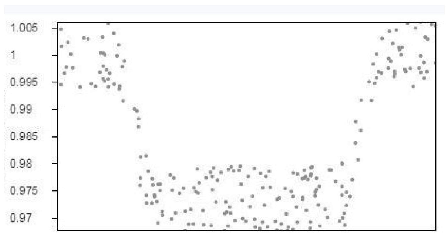
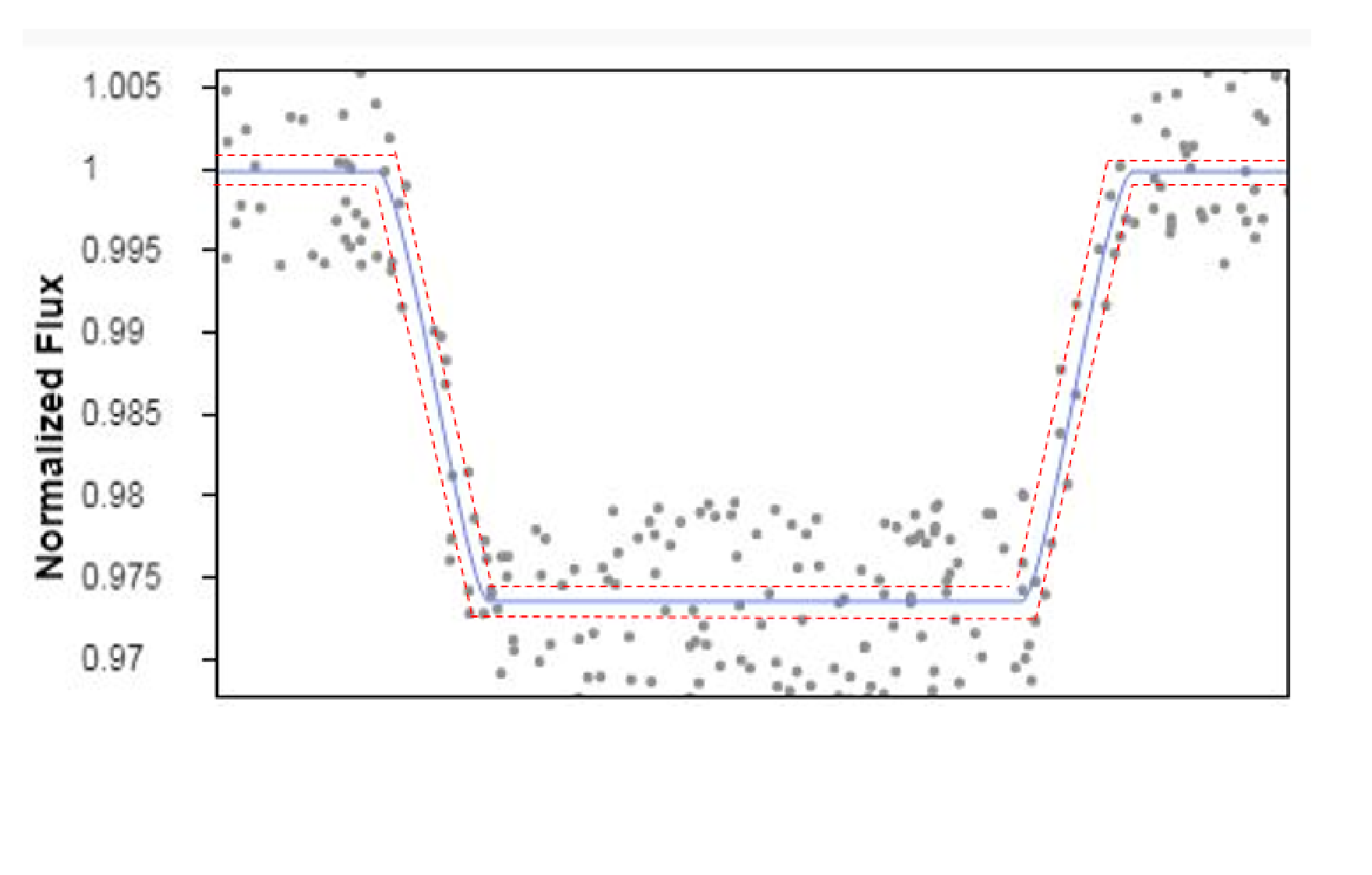
1.1 Use the given information to calculate the following quantities for the HD 209458 system:
| Luminosity of the star | Radius of the star | Mass of the star | Mean planet’s orbital radius | Radius of the planet in Jupiter’s radius |
|---|---|---|---|---|
Note: Assume that the bolometric correction for all F and G type stars is the same. [20 т.]
Part 2 (25 points). (25 т.)
The habitable zone is defined as the region in which a planet may have liquid water on its surface. This is mainly related to the amount of radiation received from the host star, which must be within some limits to ensure a favorable range of planet surface temperatures.
We define the effective flux received by a planet as , where is the star luminosity in solar units, and is the mean orbital radius in au. The minimum flux in the habitable zone can be approximated by , where , and is the equivalent flux for the case of the Sun, which along with the coefficients is given in the following table. The maximum flux for habitability, , is found with the same equation but different constants:
| Constant | ||
|---|---|---|
The table below gives real data for 7 different star-planet systems. However planet names have been changed to honour some natural sanctuaries in Colombia:
| Stellar Parameters | Planet Parameters | ||
|---|---|---|---|
| Name | |||
| 6180 | 3.68 | Tayrona | 0.04 |
| 5730 | 3.87 | Iguaque | 0.04 |
| 5980 | 4.21 | Gorgona | 0.04 |
| 5480 | 6.04 | Amacayacu | 0.08 |
| 5770 | 3.48 | Malpelo | 0.05 |
| 6130 | 3.07 | Pisba | 0.03 |
| 6140 | 3.85 | Tatamá | 0.06 |
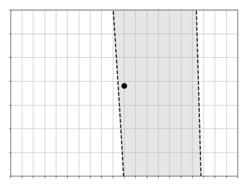
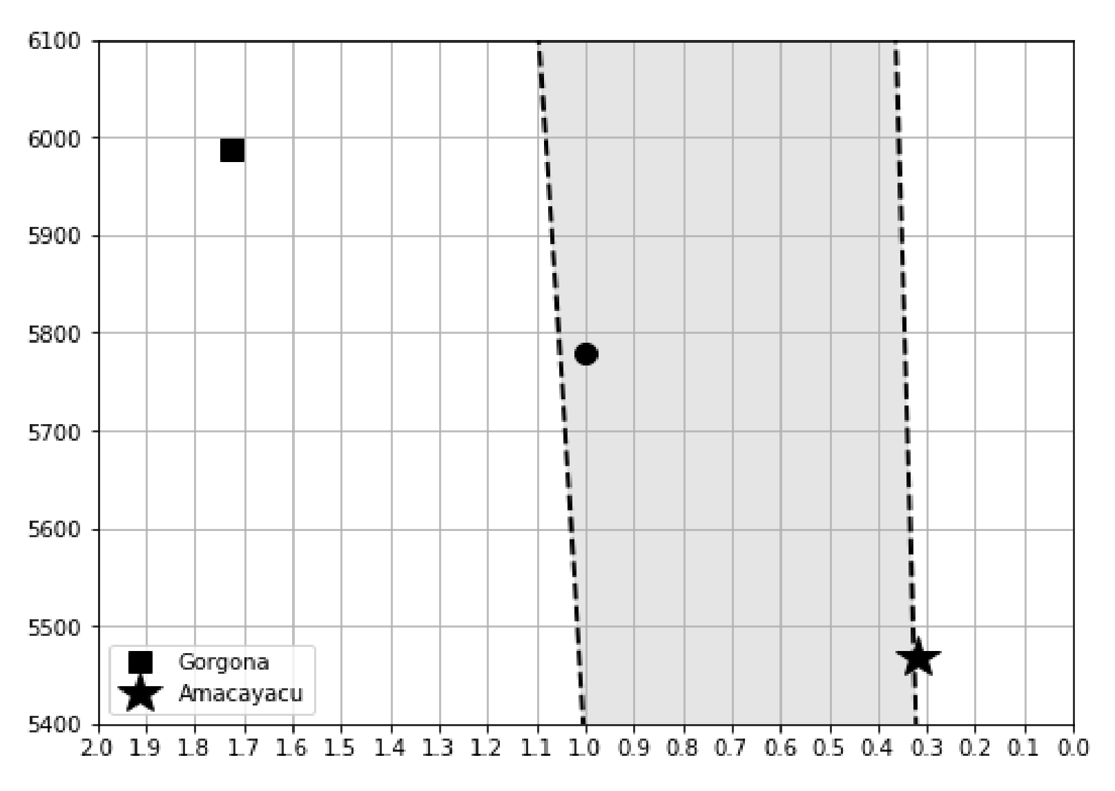
2.1 In the following figure, the vertical axis represents the effective temperature of stars, and the horizontal axis represents the effective flux received by orbiting planets. The dot marked on the graph represents planet Earth, and dashed lines mark the limits of the habitable zone.
Put numerical labels at tickmark position on both axes. Draw on the same figure the exact position where Gorgona and Amacayacu would be, as if they were also located at 1 from their corresponding stars. [15 т.]
2.2 Now considering the real orbital radius given in the table for each planet, indicate with YES or NO which of them are in the habitable zone. Show your quantitative reasoning on the working sheets.
| Planet’s Name | In habitable zone? YES / NO |
|---|---|
| Tayrona | |
| Iguaque | |
| Gorgona | |
| Amacayacu | |
| Malpelo | |
| Pisba | |
| Tatamá |
[10 т.]
Part 3 (30 points). (30 т.)
In the last page you find a list of 38 exoplanets, and the goal is to find out if low-mass exoplanets (LME) and high-mass exoplanets (HME) tend to orbit around stars with different characteristics.
3.1 To get a robust low-mass subsample one can apply a technique called “iterative sigma-clipping”. The idea is to compute the mean and the standard deviation of the masses and to exclude from the sample, those planets with masses above . Then repeat the same steps with the remaining subsample two more times. We will say that planets in the final subsample are the low-mass ones, and those excluded during the iterations, the high-mass ones. Fill the following table with the numbers you find in the process:
| Low-mass sample | Sample size | No. of planets to exclude | |||
|---|---|---|---|---|---|
| Full / Original | |||||
| subsample after 1st iteration | |||||
| subsample after 2nd iteration | |||||
| subsample after final iteration | --- | --- | --- | --- |
[10 т.]
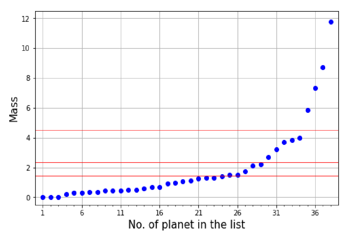
3.2 Make a plot using the X-axis for the serial number of the planets in the list , and the Y-axis for the mass of the planets. Mark 3 horizontal lines at the thresholds you found in the iterations: [5 т.]
3.3 Let’s investigate the possible difference in the effective temperatures of host stars in both groups, computing some descriptive statistics:
| Min. | 1st Quartile | Median 2nd quartile | 3rd Quartile | Max | |
|---|---|---|---|---|---|
| LME | |||||
| HME |
[10 т.]
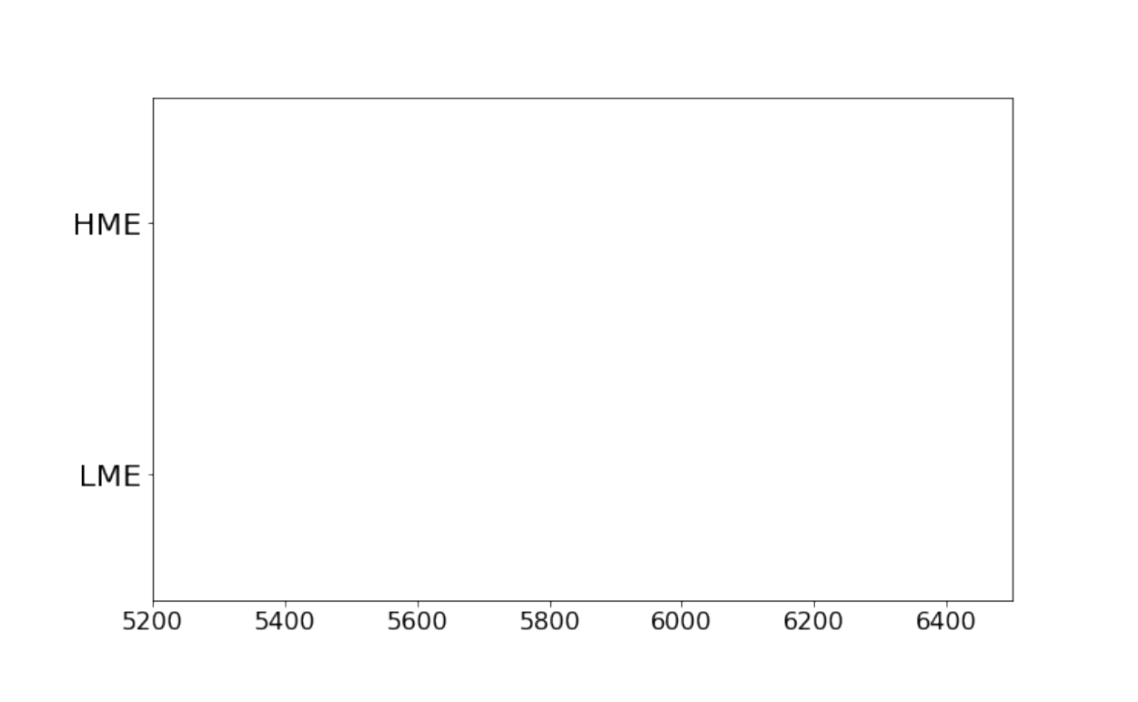
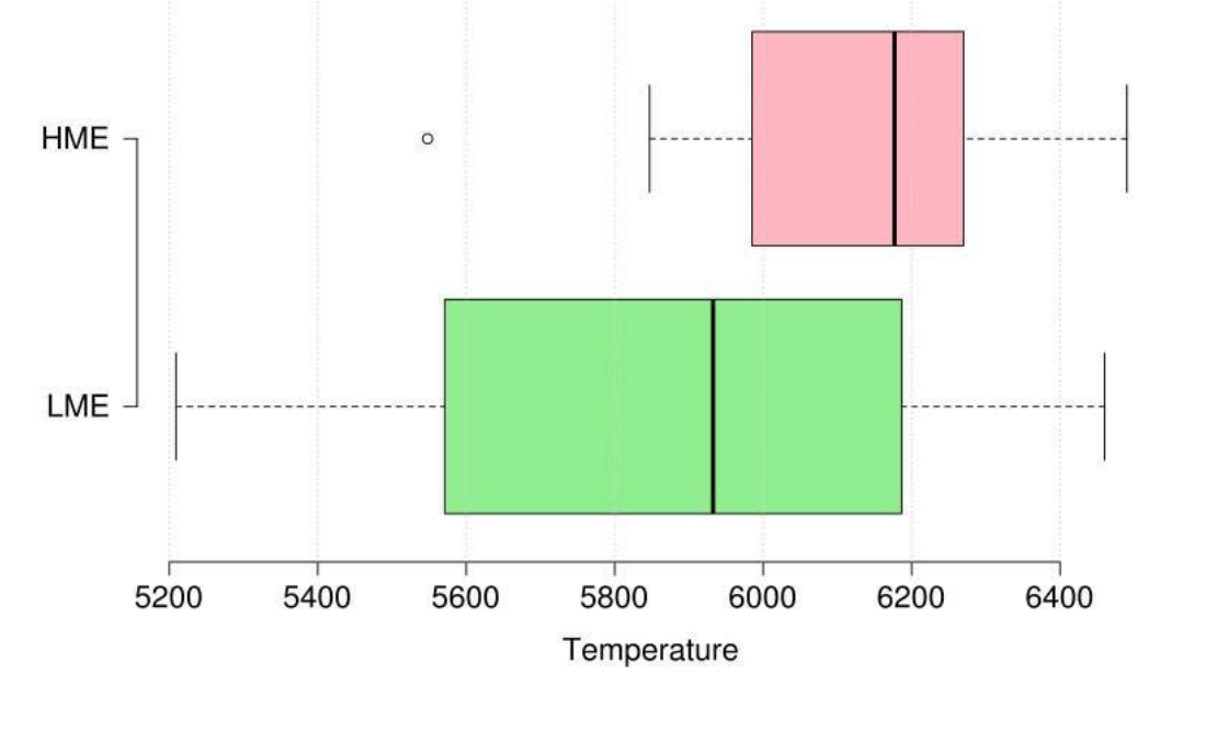
3.4 Draw boxplots summarizing the numbers you just computed. Do you see a clear difference in the temperatures of the stars orbited by low-mass and high-mass planets? Write YES or NO.
[5 т.]
| No. | Name of Planet | Planet Mass | of the Host Star |
|---|---|---|---|
| 1 | KEPLER-37 b | 0.01 | 5520 |
| 2 | KEPLER-21 b | 0.02 | 6256 |
| 3 | HD 97658 b | 0.02 | 5468 |
| 4 | HD 46375 b | 0.23 | 5345 |
| 5 | HD 219134 h | 0.28 | 5209 |
| 6 | HD 88133 b | 0.30 | 5582 |
| 7 | HD33283 b | 0.33 | 5877 |
| 8 | HD 149026 b | 0.36 | 6096 |
| 9 | BD-10 3166 b | 0.46 | 5578 |
| 10 | HD 75289 b | 0.47 | 6196 |
| 11 | HD 217014 b | 0.47 | 5755 |
| 12 | HD 2638 b | 0.48 | 5564 |
| 13 | WASP-13 b | 0.49 | 6025 |
| 14 | WASP-34 b | 0.59 | 5771 |
| 15 | HD 209458 b | 0.69 | 5988 |
| 16 | HAT-P-30 b | 0.71 | 6177 |
| 17 | WASP-76 b | 0.92 | 6133 |
| 18 | WASP-74 b | 0.97 | 5727 |
| 19 | HAT-P-6 b | 1.06 | 6442 |
| 20 | HD189733 b | 1.14 | 5374 |
| 21 | WASP-82 b | 1.24 | 6257 |
| 22 | KELT-7 b | 1.29 | 6460 |
| 23 | HD 149143 b | 1.33 | 6067 |
| 24 | KELT-3 b | 1.42 | 6404 |
| 25 | KELT-2A b | 1.49 | 6164 |
| 26 | HD86081 b | 1.50 | 6015 |
| 27 | HAT-P-7 b | 1.74 | 6270 |
| 28 | HD 118203 b | 2.14 | 5847 |
| 29 | HAT-P-14 b | 2.20 | 6490 |
| 30 | WASP-38 b | 2.71 | 6178 |
| 31 | HD17156 b | 3.20 | 5985 |
| 32 | KELT-6 c | 3.71 | 6176 |
| 33 | HD 75732 d | 3.86 | 5548 |
| 34 | HD 115383 b | 4.00 | 5891 |
| 35 | HD 120136 b | 5.84 | 6210 |
| 36 | WASP-14 b | 7.34 | 6195 |
| 37 | HAT-P-2 b | 8.74 | 6439 |
| 38 | XO-3 b | 11.79 | 6281 |
Отговори
Part 1 (20 points)., 1.1 L = 1.759 Lsun; R = 1.24 Rsun; M = 1.94 Msun; a = 0.0565 au; Rp = 1.296 RJ
Official table of results on solutions p.5; a tolerance of 5% on the final answers is accepted.
Part 2 (25 points)., 2.2 NO for all seven planets: none of the exoplanets lie in the habitable zone.
Part 3 (30 points)., 3.4 YES
Official solution: the boxplots indicate that HMEs tend to get formed around hotter stars.
Решение
Part 1. (20 т.)
Part 1. [20 points]
- With the parallax we get the distance: , [1 point] then we get the absolute magnitude using the distance modulus , [1 point] and finally we go for the luminosity as BC is assumed to be the same for all F/G stars, [2 points] by comparing with the magnitude of the Sun: . [1 point]
- We find the stellar radius from the Stephan-Boltzmann law, which in solar units leads to [2 point], i.e., . [2 points]
- Now to find the stellar mass consider the surface gravitational acceleration, which for Gauss’ law and spherical symmetry considerations is: , [1 point] then one solves for and puts it in the right units, [3 points]
- Planet’s orbital radius comes from [3 points]
- Finally, checking the dimming due to the transit this is of approximately 2.6%, which is give by the ratio between the areas of the planet disk and the stellar disk, i.e., , [2 points] leading to [2 point]
| Luminosity of the star | Radius of the star | Mass of the star | Mean planet’s orbital radius | Radius of the planet in Jupiter’s radius |
|---|---|---|---|---|
| 1.759 | 1.24 | 1.94 | 0.0565 | 1.296 |
Tolerance: of 5% on the final answers is acceptable, numbers approximated to the second digit in the partial calculations are OK.
Part 2. (25 т.)
Part 2. [25 points]
2.1) [15 points]
One first needs to calibrate the axes. The shown circle representing the Earth gives as a vertical mark in 5778 °K, and a horizontal one at . Then one need to retrieve additional data from one or more of the additional observations:
Having the temperature mark for the Sun, one can estimate , adding a second mark on the horizontal axis, so the scale of this one can be calibrated. Then one can proceed backwards, starting from a given value of or , find the corresponding temperature, so the vertical axis can be calibrated as well.
Alternatively, one can notice that the limiting curve crosses the X axis in , and look numerically for the corresponding temperature of the bottom line, thus calibrating the vertical axis. Then starting from a given temperature, one calibrates de horizontal one pivoting on / calculations as explained before.
There are several ways, some more precise than others. The student should be as careful as possible (we give small tolerance to the error in the calibrations of the axes). A tricky part is that the X-axis increases towards the left, but this is something rigorous students will discover, as there is no self-consistency otherwise. Intuition may also help if one knows that Earth is closer to the high-flux end of the Sun’s habitable zone.
The luminosity of Gorgona’s host star was found in Part A. After finding the luminosity of Amacayacu’s one the final plot looks like this:
For placing Gorgona in the right position [2 pt]
For calculating flux and placing Amacayacu in the right position [4 pt]
Grading Scheme:
TOTAL: 15 pts
Points should be given to partial achievements like:
- Horizontal axis - [4 points] – sun position - [1 point] (if did not get the 4 points)
- Vertical axis - [5 points] – sun position - [1 point] (if did not get the 5 points)
Tolerance for the position of the planets: +/- 0.025 in Seff ; +/- 25 [K] in Teff
2.2) [10 points]
NONE of the exoplanets lie in habitable zones. They orbit their stars too close, so the effective flux is many times larger than . The long-but-straightforward answer is to perform all the calculations. The elegant, clever one, is to note that Amacayacu orbits the faintest/coolest star, and it is the one farthest away, so its effective flux is the absolute minimum of the whole set. This effective flux was calculated as ~0.3 in A), assuming a distance of 1 A.U. With the real distance, 0.08 A.U, it grows by a factor , i.e., it has , but the habitable zone for this range of temperatures can not exceed , which completely closes the case.
| Name | Seff |
|---|---|
| Tayrona | 1785.994090 |
| Iguaque | 1499.270574 |
| Gorgona | 1096.175314 |
| Amacayacu | 50.794890 |
| Malpelo | 1374.231792 |
| Pisba | 5568.747040 |
| Tatama | 678.730709 |
Grading Scheme:
- [9 points] If the student argues about the case of Amacayacu as the limiting case, concluding that none of the exoplanets lie in the HZ, even if the flux is wrongly calculated. [1 point] additional for getting Amacayacu’s Seff with 10% error or less.
If the student applies an exhaustive solution:
- Each effective flux must be calculated correctly up to a 10% , giving [1 point] per each Seff. [3 pts] for explaining that all these fluxes are way too much for the HZ, which can only be awarded if all the 7 fluxes are correct. This is because it is pointless to argue about calculating numbers and comparing, if you do not calculate well.
Part 3. (30 т.)
Part 3.
3.1) [3 points] per each row. [1 point] extra for the only number in the last row.
| Low-mass sample | Sample size | μ | σ | μ + σ | No. of planets to exclude |
|---|---|---|---|---|---|
| Full / Original | 38 | 1.99 | 2.55 | 4.54 | 4 |
| 1st subsample | 34 | 1.23 | 1.11 | 2.34 | 5 |
| 2nd subsample | 29 | 0.84 | 0.61 | 1.45 | 5 |
| Final subsample | 24 | - | - | - | - |
3.2) Graph plotting technique: Coverage [1 point], labelling [1 point], correct plotting [1.5 point], horizontal lines [0.5 points x 3 ]
3.3) [1.5 points] for each quartile, [1 point] for each median. Tolerance 5%. 0.5 for each min and max
| Min. | 1st Quartile | Median | 3rd Quartile | Max | |
|---|---|---|---|---|---|
| LME | 5209 | 5574.5 | 5932.5 | 6181.75 | 6460 |
| HME | 5548 | 5992.5 | 6177.0 | 6255.0 | 6490 |
3.4) Boxplot [1.5 points] x 2, outlier [1 point]
Yes, the boxplots indicate that HMEs tend to get formed around hotter stars. [1 point]
Answer Sheets (A2-1 to A2-4)
Data Analysis 2: Stars and Exoplanets (75 points)
Part 1 (20 points).
1.1 (20.0 pt)
| Luminosity of the star | Radius of the star | Mass of the star | Mean planet’s orbital radius | Radius of the planet in Jupiter’s radius |
|---|---|---|---|---|
| a | ||||
Part 2 (25 points).
2.1 (15 pt) — the habitable-zone grid of question 2.1, printed again for the answer.
2.2 (10.0 pt)
| Planet’s Name | In habitable zone? YES / NO |
|---|---|
| Tayrona | |
| Iguaque | |
| Gorgona | |
| Amacayacu | |
| Malpelo | |
| Pisba | |
| Tatamá |
Part 3 (30 points).
3.1 (10.0 pt)
| Low-mass sample | Sample size | No. of planets to exclude | |||
|---|---|---|---|---|---|
| Full / Original | 38 | ||||
| 1st subsample | |||||
| 2nd subsample | |||||
| Final subsample | - | - | - | - |
3.2 (5.0 pt) — a blank sheet of graph paper.
3.3 (10.0 pt)
| Min. | 1st Quartile | Median 2nd Quartile | 3rd Quartile | Max | |
|---|---|---|---|---|---|
| LME | |||||
| HME |
3.4 (5.0 pt) — empty boxplot axes (HME, LME against 5200–6400), Planetary type vs host star temperature (K)
| YES | NO |
|---|---|
Оригинал в Архива: DA-2-Q.pdf · официални решения: Data Analysis Solutions.pdf · допълнителни данни: DA-2-A.pdf · допълнителни данни: DA-G.pdf · допълнителни данни: Standard-Table-of-constants.docx.pdf