Съдържание

Условие Combined original · Data Analysis - Galactic Surveys · Part 1 (35p)Combined original · Part 2 (20p)Combined original · Part 3 (20p)Отговори Решение

IOAA 2022, Анализ на данни — Задача 2. Galactic Surveys

Оригинал на условието (PDF)Съобщи за грешка

Всички материали от IOAA 2022

International Olympiad on Astronomy and Astrophysics 2022 Georgia — Data Analysis · 18 август 2022 г. · 105 т.

Условие

In Cosmology, observations of the spatial distribution of galaxies are crucial to understanding the evolution and expansion of the Universe. Numerous telescopes conduct surveys to produce catalogues of galaxies, which are then subjected to statistical analysis. Usually, galaxies form in groups, which together are part of a cluster, surrounded by a very large, spherical dark-matter halo. Most of the matter is concentrated in the centre, thus there is a high probability of having a large-mass galaxy at the centre of the halo.

In this problem, we will assume that all halos have one central galaxy and several groups of satellite galaxies, and use statistical analysis to draw inferences about the spatial distribution of galaxies.

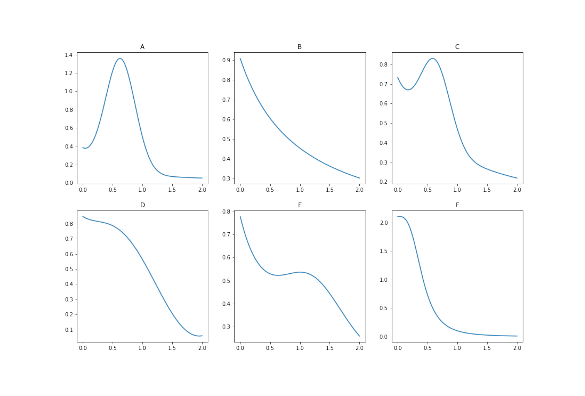
In Figure 1, you can see six different possible probability densities (A-F) for distances between galaxies. On the X axis is the separation distance between galaxies ( $a$ ), and on the Y axis is the probability density ( $f_p(a)$ ). The probability of the distance between a pair of galaxies being in the range $a$ to $a + \Delta a$ is given by

P(a) = f_p(a)\cdot\Delta a

Note that $f_p(a)$ may take values greater than 1 in some cases.

Six small plots labelled A to F of probability density versus separation from 0.0 to 2.0: A a single peak near 0.6 reaching 1.35; B a monotonic decrease from 0.9 to 0.3; C a dip near 0.2 then a peak near 0.6 at 0.83, falling to 0.22; D a slow then faster decrease from 0.85 to 0.06; E a fall from 0.78 to 0.52, a plateau with a slight bump near 1.0, then a fall to 0.26; F a steep fall from 2.1 to near 0. — Figure 1: Probability density of all possible galaxy pairs

i	$x$ (Mpc)	$y$ (Mpc)	$z$ (Mpc)	$N_i$
C	8.300	6.200	1.100	Central
1	8.401	6.309	1.394	291
2	9.883	7.189	1.506	170
3	8.883	6.413	2.226	253
4	8.444	6.569	2.439	8
5	7.782	6.048	-0.358	72
6	8.780	6.305	2.463	120
7	7.990	5.881	0.532	302
8	8.540	6.388	0.369	52
9	7.975	6.030	1.216	28
10	7.072	5.431	0.488	40
11	8.037	5.965	0.615	72
12	8.681	6.483	0.734	379
13	7.115	5.259	1.403	82
14	9.587	7.130	0.322	62
15	8.193	6.104	0.915	305
16	7.613	5.847	1.666	293

Table 1: Coordinates of galaxy groups

Part 1 (60pt)

Table 1 gives the observational data of a single dark matter halo in the form of Cartesian coordinates of 16 satellite groups and the coordinates of the central galaxy which is given in the first row. $i^{th}$ group consists of $N_i$ galaxies. The origin of this coordinate system is the Earth. For simplicity, we assume that a group of galaxies means a collection of galaxies with almost the same coordinates.

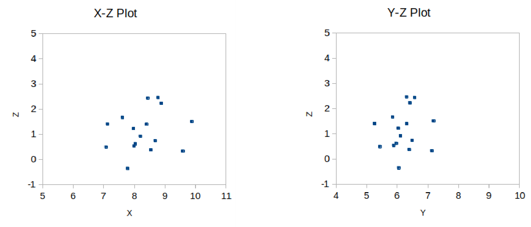
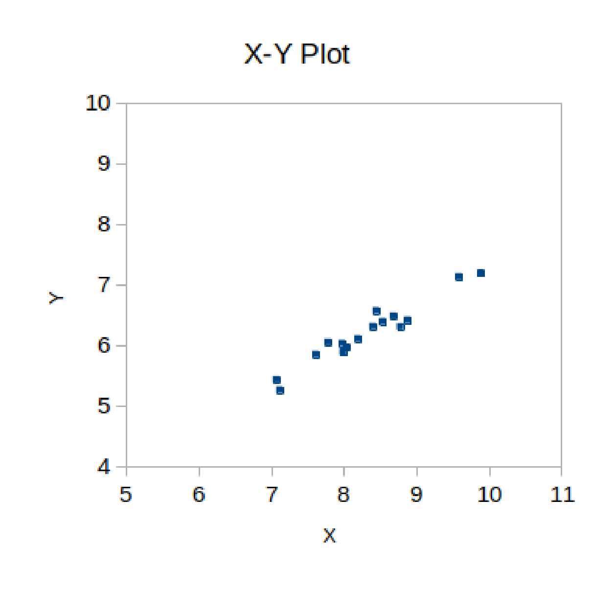
Part 1 (a) The distribution of the satellite groups in $X-Z$ plane and $Y-Z$ plane has been plotted for you. Plot the distribution in the $X-Y$ plane on millimeter paper. [6 т.]

Two scatter plots of the satellite groups: X-Z Plot (X from 5 to 11, Z from -1 to 5) and Y-Z Plot (Y from 4 to 10, Z from -1 to 5).

Part 1 (b) Given that this cluster of galaxies is shaped like a disk and our line of sight is in the plane of the disk, find the unit vector in the direction of the normal to the disk. [4 т.]

Part 1 (c) Let us define a new coordinate system centred on the central galaxy, defining our line of sight from the Earth to the central galaxy as the $X'$ axis and the normal to the disk as the $Z'$ axis. Find the unit vectors for this coordinate system. [2 т.]

Part 1 (d) Convert the given Cartesian coordinates to the new $X'Y'Z'$ coordinates. Calculate: $X'$ , $Y'$ , $Z'$ . [24 т.]

Part 1 (e) Write the equations necessary to convert the new $X'Y'Z'$ Cartesian coordinates into spherical coordinates centred on the central galaxy. $\theta$ coordinate has been already calculated for you below. Calculate $R$ and $\phi$ . [11 т.]

i	$\theta$
1	1.652
2	1.490
3	1.432
4	1.721
5	1.692
6	1.430
7	1.474
8	1.580
9	1.723
10	1.646
11	1.519
12	1.569
13	1.542
14	1.557
15	1.516
16	1.705

Note: in spherical coordinates, one uses the coordinates $R$ , $\theta$ and $\phi$ , where $R$ is the radial distance, $\phi$ is the azimuthal angle measured anti-clockwise from $X'$ axis (from 0 to $2\pi$ ) and $\theta$ is the polar angle (from 0 to $\pi$ ), i.e. angle relative to $Z'$ axis.

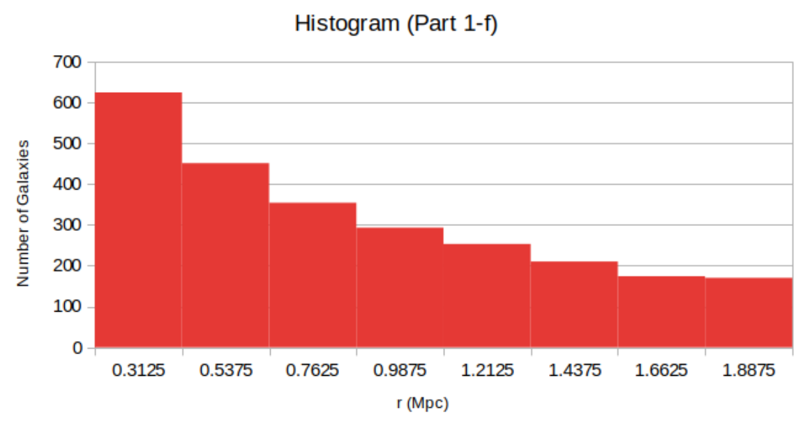
Part 1 (f) Plot a histogram (on millimeter paper) showing the number of satellite galaxies at different radial distances from the central galaxy. Use 8 equally sized bins for radial distances, with $0.2\,\mathrm{Mpc}$ to $2\,\mathrm{Mpc}$ as the total range of the histogram. [9 т.]

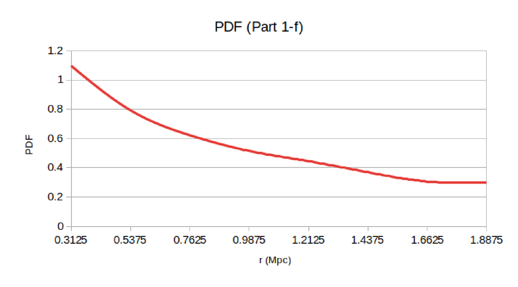
Part 1 (g) The histogram must be also converted into a probability density. On the right hand side of the vertical axis of the histogram you plotted, add markings for the re-scaled vertical axis appropriated for the probability density. You will use this probability density data in Part 3. [4 т.]

Part 2 (17pt)

The coordinates in the Table above are determined using distances obtained by the redshift method. It is well-known that while measuring distance to any galaxy with the redshift method, errors might occur because of the orbital motion of the galaxies. Now, we will try to correct for these errors.

Assume that the central galaxy has an effective mass of $10^{10}M_{\odot}$ , all satellite galaxies move in circular orbits around the central galaxy and interactions between any two satellite galaxies can be ignored.

Part 2 (a) Use the data in Table 1 of the question sheet to obtain a histogram of number of galaxies against the $\phi$ azimuthal angle (take the width of the bins as $60^{\circ}$ ). The angle distribution is expected to be uniform, but it is not. Calculate the standard deviation for this data. [5 т.]

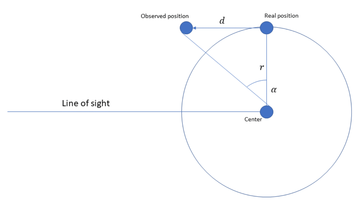
Part 2 (b) The two bins centred along the $Y'$ axis show unusually low number of galaxies as the orbital velocities of satellite galaxies in these bins are almost parallel to our line of sight and hence there is maximum error in their distance estimated by the redshift method. Derive an expression for the correction in each azimuthal angle.

Note: You may assume that the distance from the central galaxy ( $R$ ) doesn’t change significantly because of this correction. [4 т.]

Part 2 (c) Calculate corrected value of the azimuthal angles for each data row and recalculate the histogram and standard deviation of its values. [8 т.]

Part 3 (28pt)

So far, we have only calculated the central galaxy – satellite galaxy histogram for a single halo. It is time to move on to calculating other relations.

The same observations and data analysis has been carried out for different halos and their central galaxies. Suppose we have 500 halos, thus, 500 central galaxies ( $N_C = 500$ ). Take that the average number of satellite galaxies in each halo is 1000 ( $N_S = 1000$ ).

Part 3 a) Calculate the following quantities:

(1) $N_{CC}$ , total number of pairs of central galaxies

(2) $N^*_{CS}$ , total number of central galaxy - satellite pairs such that the galaxies in the pair belong to the same halo.

(3) $N_{CS}$ , total number of central galaxy - satellite pairs such that the galaxies in the pair belong to two separate halos.

(4) $N^*_{SS}$ , total number of satellite - satellite galaxy pairs such that the galaxies in the pair belong to the same halo.

(5) $N_{SS}$ , total number of satellite - satellite galaxy pairs such that the galaxies in the pair belong to two separate halos. [5 т.]

The table below gives the probability density values for different distances between central galaxies in different dark matter halos (CC). You should note this data is not real and doesn’t represent the results of the real observations. Dark matter halos do not intersect. But for simplicity we will use this data.

$R$ (Mpc)	$\rho_{CC}$
0.3125	0.406
0.5375	0.808
0.7625	1.341
0.9875	1.134
1.2125	0.479
1.4375	0.143
1.6625	0.073
1.8875	0.060

We can calculate all probability densities using the given Center-Center (CC) data and the same halo Center-Satellite ( $CS^*$ ) data that we have calculated in Part 1. We use following relations:

\rho^*_{SS}(R) = c_1 R\left[\rho^*_{CS}(R)\right]^2

\rho_{CS}(R) = c_2 R\left[\rho^*_{CS}(R)\right]^2\sqrt{\rho_{CC}(R) + 1}

\rho_{SS}(R) = c_3 R\left[\rho^*_{CS}(R)(\rho_{CC}(R) - 5)\right]^2

Where $c_1$ , $c_2$ and $c_3$ are normalization constants and should be found for each probability density.

Part 3 b) Calculate normalised $\rho^*_{SS}(R)$ , $\rho_{CS}(R)$ and $\rho_{SS}(R)$ . [15 т.]

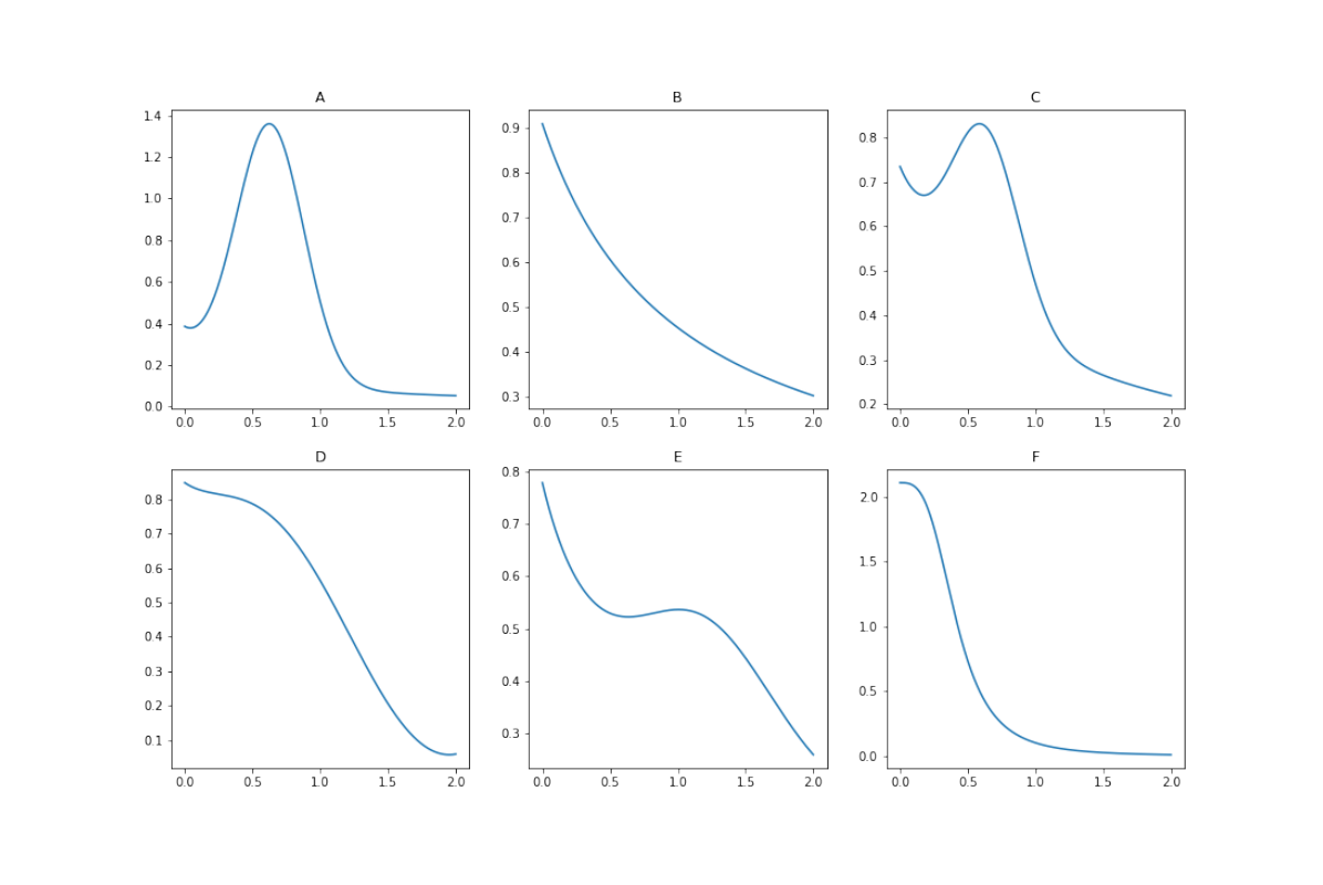
Part 3 c) Calculate the final probability density of all galaxy pairs, that combines all the distributions above with appropriate weights. Which one of 6 graphs on Figure 1 best represents this probability density? [8 т.]

Combined original · Data Analysis - Galactic Surveys · Part 1 (35p)

Additional original source: Data Analysis Problems & Solutions.pdf. The complete differing version below retains its own requests, coordinate convention, marking scheme and figures. The dated question and matching solution version above stays unchanged. No chronology is printed on this combined source.

Source note. The separate Table 1 answer-sheet form cited in (c) and (d) was not among the obtainable original files. The source-specific coordinate signs, pair counts, degree units and differing numerical keys below are retained as printed.

In Cosmology, observations of galaxy groups is very important for the study and verification of complex theory models, Universe expansion, and its behaviour analysis. There are numerous telescopes used only for galactic surveys and making special statistical analysis. The product of all this are the catalogues of galaxies, which are the result of this observations and complex computational analysis.

Usually, galaxies form in groups inside very large dark matter Halos (that have a spherical shape). The most matter is concentrated in the center, thus having a central large-mass galaxy there is with high probability. In these problem, we will assume that all Halos have one central galaxy and several satellite galaxies.

As one can guess, all of these requires a large amount of computational power: To distinguish galaxies, process corrected coordinates with redshifts and other methods, etc. The complex statistical analysis involves calculating correlation functions for galaxy groups, which is making a histogram for distances between all possible two galaxy pairs. The main goal of this problem is to do theoretical statistical analysis of the observational data and figure out what kind of galaxy groups have been observed. Having a theoretical model that can deduce the characteristics of a galaxy groups with few observations is very useful for scientists and saves lots of computational time and possible errors following those kind of data analysis.

In Figure 1, you can see the probability densities of different galaxy groups. On X axis is the distance, and on Y axis is probability density. There are six galaxy cluster types (A-F) with corresponding densities. The goal of this problem will be to determine what kind of Dark matter Halo groups we are observing.

Figure 1: Probability density of all possible galaxy pairs (from different/same dark matter Halos)

Part 1 (35p)

You are given Table 1. that represents the data from observations. From other data and observations it was concluded that all these galaxies belong to the same dark matter halo. You can see the coordinates of satellite galaxies. The coordinate for the central galaxy is 8.300; 6.200; 1.100. Additional column represents the number of galaxies spotted very near to that points. For simplicity, you can assume that the coordinates are the same for them. These coordinates are given in Cartesian coordinate system center of which coincides to the observer on Earth.

i	x (MPC)	y (MPC)	z (MPC)	N (Number of galaxies)
1	8.401	6.309	1.394	291
2	9.883	7.189	1.506	170
3	8.883	6.413	2.226	253
4	8.444	6.569	2.439	8
5	7.782	6.048	-0.358	72
6	8.780	6.305	2.463	120
7	7.990	5.881	0.532	302
8	8.540	6.388	0.369	52
9	7.975	6.030	1.216	28
10	7.072	5.431	0.488	40
11	8.037	5.965	0.615	72
12	8.681	6.483	0.734	379
13	7.115	5.259	1.403	82
14	9.587	7.130	0.322	62
15	8.193	6.104	0.915	305
16	7.613	5.847	1.666	293

Before we start converting Cartesian coordinates to spherical we need to find appropriate local coordinate system with origin in the center of the halo.

(a) Plot all the pairs of Cartesian coordinates on the separate graphs. Given the fact that this halo is shaped like a disk find the direction of its normal. [4 т.]

(b) Write down the unit vectors of local coordinate system. Choose appropriate orientation and take $X'$ axis such that coincides the line of sight. [3 т.]

(c) Convert the given Cartesian coordinates to the local $X'Y'Z'$ coordinates. Fill in the values of Table 1 (a separate sheet is given in the answer sheets): $X'$ , $Y'$ , $Z'$ . [8 т.]

(d) Convert the local Cartesian coordinates into spherical (take the central galaxy as the center of the coordinate system, $\phi$ is calculated relative to $X'$ axis and $\theta$ - relative to $Z'$ axis). Fill in the other values of Table 1 (a separate sheet is given in the answer sheets): $r$ , $\theta$ , $\phi$ . [8 т.]

(e) Plot the histogram (parameter dependence on total number of data points that fall in a given limits) with 8 bins of Satellite galaxy distances from the central Galaxy. Take 0.2-2 MPC as the histogram range. The histogram has to be also converted into probability density function. Note: The probability density function is the probability at a given point. You can avoid plotting two separate graphs by just noting other limits of Y axis in case of probability function. [6 т.]

(f) Theoretically the histogram is given by the following equation

H(r)=\frac1{A+B\cdot r}\qquad (1)

Linearize the given dependence and find values $A$ and $B$ from the graph. [6 т.]

Combined original · Part 2 (20p)

It is well-known that while measuring distance to an object with redshift method (large relative velocity due to the expansion of the universe) errors might occur because of the motion of the galaxies. The aim of this chapter is to correct these errors.

Assume that the central galaxy has a mass of $10^{10}M_{Sun}$ , all satellite galaxies move in circular orbits and interactions between them is negligible.

(a) Use the data filled with you in Table 1 to plot the histogram of polar angle (take the width of histogram bins as 60 degrees). The angle distribution should be uniform, but it is not. Calculate the square deviation from the uniform value. [6 т.]

(b) The galaxies originally in 60-120 and 240-300 bins would need most correction since they are the ones which move along the line of sight. Assume that the angular coordinates coincide with the center of the corresponding bin (90 and 270 in our case) and write the expression as a function of distance from the center which describes change of polar angles caused by circular motion of the galaxies. Hint: You can assume that the distance from the centre doesn’t change significantly because of this correction. [6 т.]

(c) Using the result of previous task correct the angles used in the last histogram. Plot the new histogram (probability dependence on distance) with the corrected data. Calculate the square deviation from the uniform value. [8 т.]

Combined original · Part 3 (20p)

We have only calculated the central galaxy - satellite (from the same galaxy) histogram. It is time to move on to calculating other relations.

The same observations and data analysis has been carried out for different Halos and their central galaxies. The data for Figure 2. histogram only includes the distribution probability density function of the distances between central galaxies in different dark matter Halos. Suppose we have 500 Halos, thus 500 central galaxies ( $N_C=500$ ). Take that the average number of satellite in one Halo is 1000 ( $N_S=1000$ ).

(a) Calculate the following quantities:

$N_{CC}$ , total number of central galaxy pairs
$N^*_{CS}$ , total number of central galaxy - satellite pairs in the same Halo
$N_{CS}$ , total number of central galaxy - satellite pairs in different Halos
$N^*_{SS}$ , total number of satellite - satellite galaxy pairs in the same Halo
$N_{SS}$ , total number of satellite - satellite galaxy pairs in different Halos [3 т.]

Below is given the table for probability density values for different distances between central galaxies in different dark matter Halos.

r (MPC)	$\rho$
0.3125	0.406
0.5375	0.808
0.7625	1.341
0.9875	1.134
1.2125	0.479
1.4375	0.143
1.6625	0.073
1.8875	0.060

We can calculate all probability densities using the given Center-Center data and Center-Satellite data which you calculated in part 1. The relations are following:

\rho^*_{SS}(r)=c_1\rho^*_{CS}(r)^2r\qquad (2)

\rho_{CS}(r)=c_2\rho^*_{CS}(r)^2r\sqrt{\rho_{CC}(r)+1}\qquad (3)

\rho_{SS}(r)=c_3\rho^*_{CS}(r)^2r(\rho_{CC}(r)-5)^2\qquad (4)

Where $c_1$ , $c_2$ and $c_3$ are normalization constant and should be found for each density.

(b) Calculate and plot $\rho^*_{SS}(r)$ , $\rho_{CS}(r)$ , and $\rho_{SS}(r)$ . [10 т.]

(c) Plot the final probability density of all galaxy pairs. Which one of 6 graphs on Figure 1 is most similar to you plot? [7 т.]

Отговори

Решение

Part 1

Part (a)

Indicated $X$ axis, written few numbers on the axis and written proper units 0.5pt. Indicated $Y$ axis, written few numbers on the axis and written proper units 0.5pt. Used $70-100$ percent of the graphing paper 2pt, for $50-70$ percent 1.5pt, for $30-50$ percent 1pt, for $30-50$ percent 0.5pt. If drawn $14-16$ points 3pt, If $10-14$ then 2pt, for 6-10 1pt and for $0-6$ 0pt

Scatter plot X-Y Plot of the satellite groups, X from 5 to 11 and Y from 4 to 10; the points lie along a rising line from about (7, 5.3) to (9.9, 7.2). — X-Y Plot

Part (b)

The normal to the disk also lies in $XY$ plane. The line of sight (which we can take as $X'$ axis) is also perpendicular to the normal. Thus, it can be calculated by normalizing $8.300\hat{i} + 6.200\hat{j} + 1.100\hat{k}$ . So

\hat{x'} = 0.79668\hat{i} + 0.59511\hat{j} + 0.10558\hat{k} \qquad \mathbf{1.0}

(here the coefficient of $\hat{k}$ is unimportant). $Z'$ axis lays in XY plane and is perpendicular to $X'$ . So

\vec{z'} = \hat{x'}\times\hat{k} = 0.59511\hat{i} - 0.79668\hat{j} \qquad \mathbf{2.0}

|\vec{z'}| = 0.99441 \qquad \mathbf{0.5}

\therefore \hat{z'} = 0.59845\hat{i} - 0.80116\hat{j} \qquad \mathbf{0.5}

[Alternative way: Calculate the equation of line of galaxies using linear regression 2pt, construct perpendicular line 1pt, normalise 1pt]

Part (c)

\hat{x'} = 0.79668\hat{i} + 0.59511\hat{j} + 0.10558\hat{k}

\hat{z'} = 0.59845\hat{i} - 0.80116\hat{j}

\hat{y'} = \hat{z'}\times\hat{x'} = -0.084589\hat{i} - 0.063187\hat{j} + 0.99441\hat{k} \qquad \mathbf{2.0}

Part (d)

Each coordinate in $X'Y'Z'$ system can be found by following equations

x' = \hat{x'}\cdot(\vec{r} - \vec{r_c})

y' = \hat{y'}\cdot(\vec{r} - \vec{r_c})

z' = \hat{z'}\cdot(\vec{r} - \vec{r_c})

8/3 points for each formula, here, $\vec{r}$ is coordinate of a satellite galaxy and $\vec{r_c}$ is coordinate of the central galaxy.

These values are calculated in the following table (1.0 for each row):

	$x - x_c$	$y - y_c$	$z - z_c$	$x'$	$y'$	$z'$
1	0.101	0.109	0.294	0.1766	0.2769	-0.02688
2	1.583	0.989	0.406	1.893	0.2073	0.1550
3	0.583	0.213	1.126	0.7101	1.057	0.1783
4	0.144	0.369	1.339	0.4757	1.296	-0.2094
5	-0.518	-0.152	-1.458	-0.6571	-1.396	-0.1882
6	0.480	0.105	1.363	0.5888	1.308	0.2031
7	-0.310	-0.319	-0.568	-0.4968	0.5184	0.07005
8	0.240	0.188	-0.731	0.2259	0.7591	-0.006988
9	-0.325	-0.170	0.116	-0.3478	0.1536	-0.05830
10	-1.228	-0.769	-0.612	-1.500	-0.4561	-0.1188
11	-0.263	-0.235	-0.485	-0.4006	-0.4452	0.03088
12	0.381	0.283	-0.366	0.4333	-0.4141	0.001284
13	-1.185	-0.941	0.303	-1.4721	0.4610	0.04472
14	1.287	0.930	-0.778	1.4966	-0.9413	0.02514
15	-0.107	-0.096	-0.185	-0.162	-0.169	0.0129
16	-0.687	-0.353	0.566	-0.6976	0.6433	-0.1283

Part (e)

Spherical coordinates can by calculated by following relations:

R = \sqrt{x'^2 + y'^2 + z'2} \qquad \mathbf{1.0}

\phi = \tan^{-1}\left(\frac{y'}{x'}\right) \qquad \mathbf{1.0}

\theta = \cos^{-1}\left(\frac{z}{r}\right) \qquad \mathbf{1.0}

Calculated values are given in the following table (0.5 for each row):

	$R$	$\phi$	$\phi$ (deg)	$\theta$
1	0.3294	1.004	57.51°	1.652
2	1.910	0.1091	6.25°	1.490
3	1.286	0.9792	56.10°	1.432
4	1.396	1.219	69.84°	1.721
5	1.555	4.273	244.80°	1.692
6	1.449	1.148	65.77°	1.430
7	0.7214	3.948	226.22°	1.474
8	0.7920	5.002	286.57°	1.580
9	0.3847	2.726	156.18°	1.723
10	1.573	3.437	196.91°	1.646
11	0.5997	3.980	228.02°	1.519
12	0.5993	5.520	316.30°	1.569
13	1.543	2.838	162.61°	1.542
14	1.768	5.722	327.83°	1.557
15	0.2343	3.948	226.20°	1.516
16	0.9576	2.397	137.32°	1.705

Part (f)

To divide the range in 8 equal bins, we must take $r_{bin} = 0.225\,\mathrm{Mpc}$ . 1.0

By calculating bin ranges and counting the number of satellite galaxies in each bin, we get: (0.5 for each row)

	Bin Center	Bin range	$n$
1	0.3125 Mpc	0.200 Mpc–0.425 Mpc	624
2	0.5375 Mpc	0.425 Mpc–0.650 Mpc	451
3	0.7625 Mpc	0.650 Mpc–0.875 Mpc	354
4	0.9875 Mpc	0.875 Mpc–1.10 Mpc	293
5	1.2125 Mpc	1.10 Mpc–1.325 Mpc	253
6	1.4375 Mpc	1.325 Mpc–1.55 Mpc	210
7	1.6625 Mpc	1.55 Mpc–1.775 Mpc	174
8	1.8875 Mpc	1.775 Mpc–2.00 Mpc	170

For plotted histogram 0.5 for each data point.

Bar histogram of Number of Galaxies versus r (Mpc) with bins centred at 0.3125 to 1.8875: 624, 451, 354, 293, 253, 210, 174, 170. — Histogram (Part 1-f)

Part (g)

The sum of the area under the histogram is,

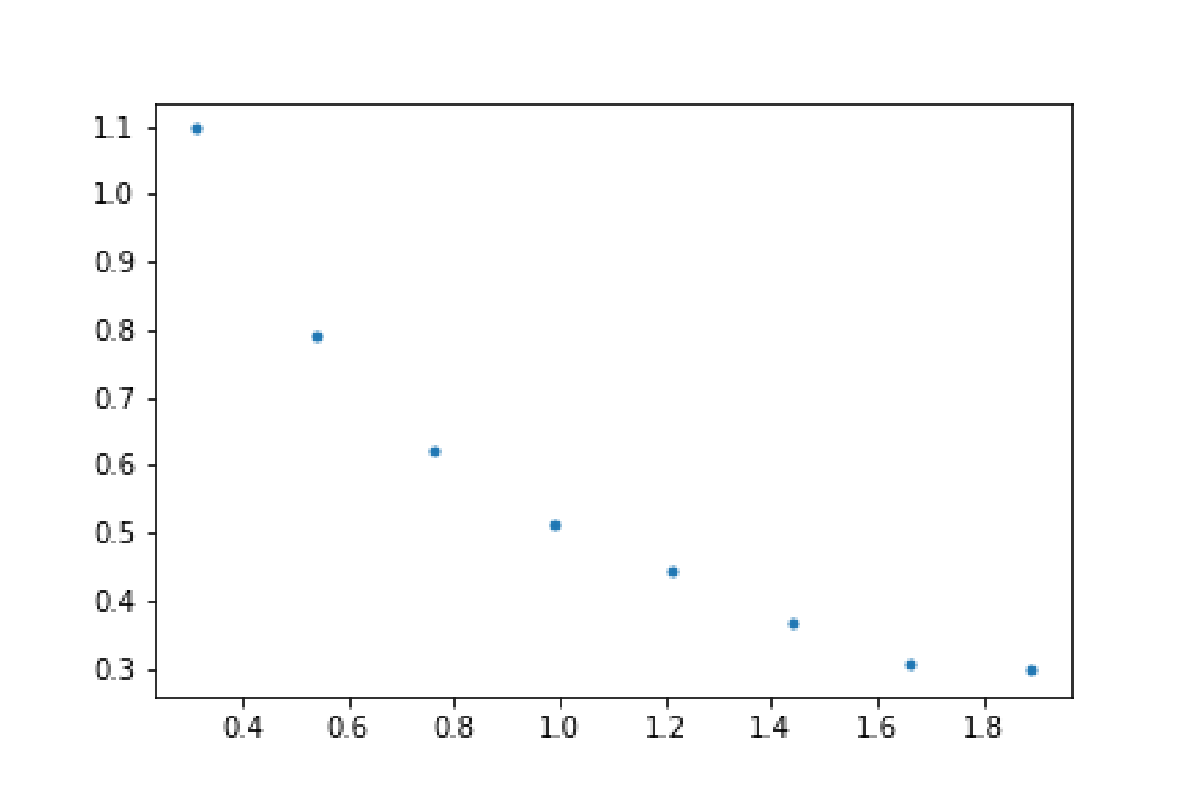
I = \sum_{i=1}^{8} n_i\cdot r_i = r_{bin}\sum_{i=1}^{8} n_i = 0.225\times 2529

I = 569.025 \qquad \mathbf{2.0}

After dividing each $n_i$ by $I$ we get (0.25 for each row):

	Bin Center	$n_i$	Probability Density
1	0.3125 Mpc	624	1.097
2	0.5375 Mpc	451	0.793
3	0.7625 Mpc	354	0.622
4	0.9875 Mpc	293	0.515
5	1.2125 Mpc	253	0.445
6	1.4375 Mpc	210	0.369
7	1.6625 Mpc	174	0.306
8	1.8875 Mpc	170	0.299

Plotting this data gives us (no separate points)

Line graph PDF versus r (Mpc) from 0.3125 to 1.8875, decreasing smoothly from about 1.1 to 0.3. — PDF (Part 1-f)

Part 2

Part (a)

Making $60^{\circ}$ bins for $\phi$ (0.5 for each row),

	Center of the bin	Number of galaxies
1	30	714
2	90	128
3	150	403
4	210	719
5	270	124
6	330	441

The expected value for each bin, in case of uniform distribution is $\bar{n} = 2529/6 = 421.5$ . Thus, the standard deviation will be

\sigma_1 \approx 264 \qquad \mathbf{2.0}

Bar histogram of Number of Galaxies versus Azimuthal Angle with bins centred at 30, 90, 150, 210, 270, 330: 714, 128, 403, 719, 124, 441. — Histogram (Part 2-a)

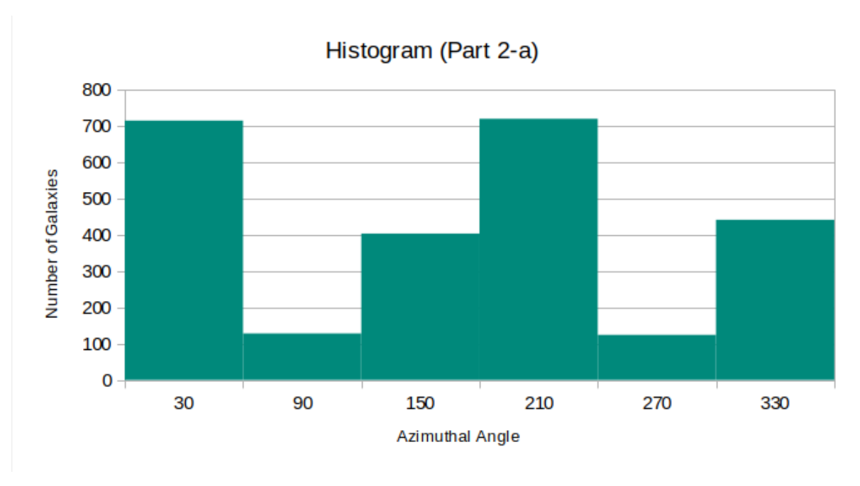
The histogram looks like (no separate points)

Part (b)

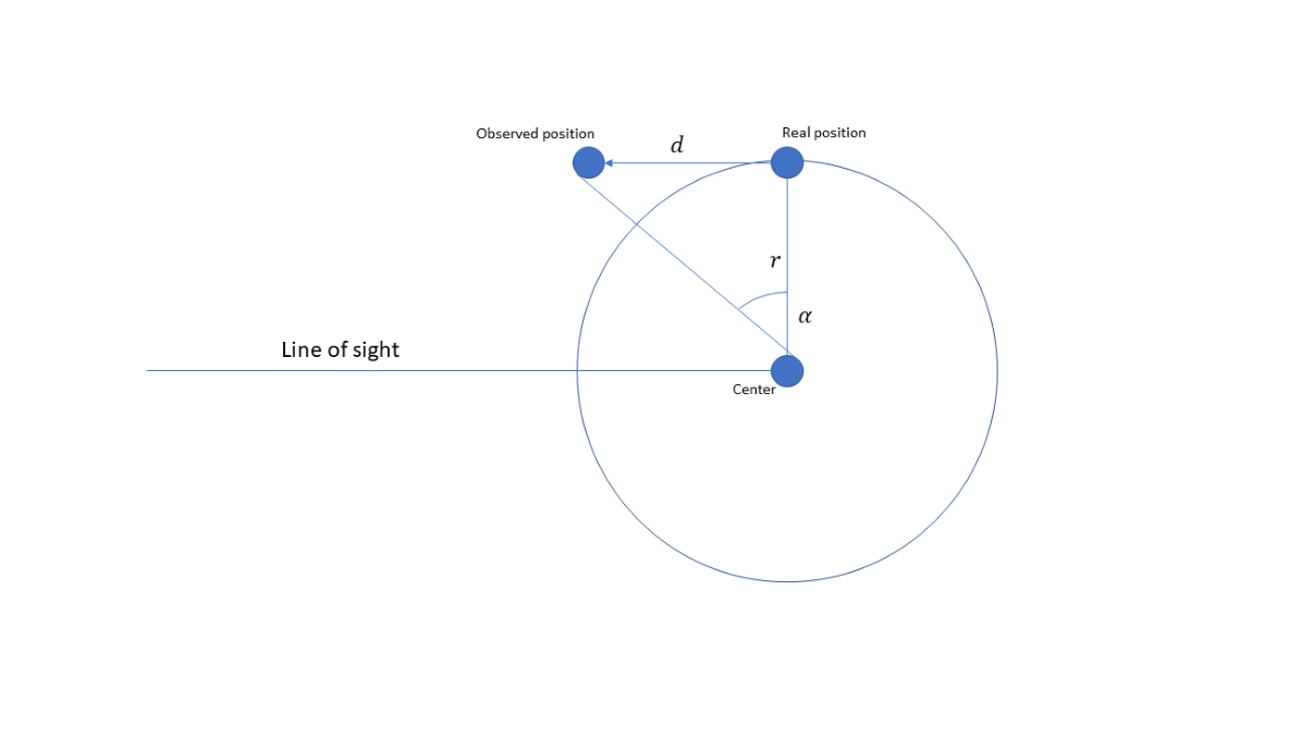
A galaxy with the orbital radius $r$ around central mass $M$ is shown in the drawing

Drawing of a circular orbit of radius r around the Center; the Line of sight is horizontal; the Real position is at the top of the circle and the Observed position is shifted by d to the left; α is the angle at the centre between the two positions.

v_{\mathrm{orbital}} = \sqrt{\frac{GM}{r}} \qquad \mathbf{1.0}

d_{\mathrm{uncorrected}} = \frac{v_{\mathrm{measured}}}{H_0} = \frac{(v_{\mathrm{redshit}} + v_{\mathrm{orbital}})}{H_0}

\therefore \Delta d = \frac{v_{\mathrm{orbital}}}{H_0} = \frac{1}{H_0}\sqrt{\frac{GM}{r}} \qquad \mathbf{1.5}

\Delta\phi = \tan^{-1}\left(\frac{\Delta d}{r}\right) = \tan^{-1}\left(\frac{1}{H_0}\sqrt{\frac{GM}{r^3}}\right) \qquad \mathbf{1.5}

[Alternative Solution:

v_{orb} = \sqrt{\frac{GM}{r}} \qquad \mathbf{1.0}

d = \frac{v}{H_0} = \frac{v_{rredshift} - v_{orb}cos(\phi)}{H_0} \qquad \mathbf{1.0}

\Delta d = r\cdot sin(\Delta\phi) = \frac{v_{orb}\cdot cos(\Delta\phi)}{H_0} \qquad \mathbf{1.0}

tan(\Delta\phi) = \frac{v_{orb}}{r\cdot H_0} \qquad \mathbf{0.5}

\Delta\phi = tan^{-1}\left(\frac{v_{orb}}{r\cdot H_0}\right) \qquad \mathbf{0.5}

]

Part (c)

We calculate $\Delta\phi$ for each value of $r$ and add it to the respective $\phi$ (choice of addition / subtraction is dependent on sign convention. Students should realise that some of the galaxies should get added to bins 2 and 5).

The table looks like this (0.25 for each row)

	$\phi_1$	$\Delta\phi$	$\phi_{\mathrm{corrected}}$	Number of galaxies
1	57.51°	27.36°	83.87°	291
2	6.25°	2.03°	8.28°	170
3	56.10°	3.68°	59.78°	253
4	69.84°	3.25°	73.09°	8
5	244.80°	2.77°	247.57°	72
6	65.77°	3.08°	68.84°	120
7	226.22°	8.69°	234.92°	302
8	286.57°	7.57°	294.14°	52
9	156.18°	21.44°	177.62°	28
10	196.91°	2.72°	199.63°	40
11	228.02°	11.41°	239.43°	72
12	316.30°	11.42°	327.72°	379
13	162.61°	2.80°	165.41°	82
14	327.83°	2.28°	330.11°	62
15	226.20°	39.56°	265.77°	305
16	137.32°	5.71°	143.03°	293

New corrected distribution looks like this (0.5 for each correct n):

	Center of the bin	Number of galaxies
1	30	423
2	90	419
3	150	403
4	210	414
5	270	429
6	330	441

Thus, the standard deviation will be

\sigma_1 \approx 13 \qquad \mathbf{1.0}

Bar histogram of Number of Galaxies versus Azimuthal Angle after correction, bins 30 to 330 all about 400–440 (423, 419, 403, 414, 429, 441). — Histogram (Part 2-c)

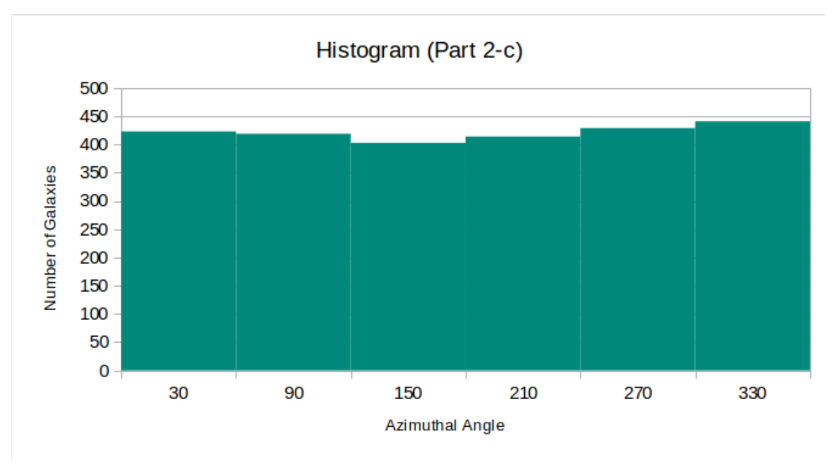
The histogram looks like (no separate points)

Part 3

Part (a)

With simple combinatorics one can get:

N_{CC} = \frac{1}{2}N_C(N_C - 1) = 124750 \qquad \mathbf{1.0}

N^*_{CS} = N_C N_S = 500000 \qquad \mathbf{1.0}

N_{CS} = N_C(N_C - 1)N_S = 249500000 \qquad \mathbf{1.0}

N^*_{SS} = \frac{1}{2}N_C N_S(N_S - 1) = 249750000 \qquad \mathbf{1.0}

N_{SS} = \frac{1}{2}N_C(N_C - 1)N_S^2 = 124750000000 \qquad \mathbf{1.0}

Part (b)

We can calculate all probability densities using center-center and center-satellite densities. Non-normalized values (with $c_1 = c_2 = c_3 = 1$ ) (1 pt) are calculated in the following table (0.5 for each correct value):

	$r$	$\rho^*_{CS}$	$\rho_{CC}$	$\rho^*_{SS}$	$\rho_{CS}$	$\rho_{SS}$
1	0.3125	1.097	0.406	0.376	0.446	7.931
2	0.5375	0.793	0.808	0.338	0.454	5.934
3	0.7625	0.622	1.341	0.295	0.452	3.951
4	0.9875	0.515	1.134	0.262	0.382	3.913
5	1.2125	0.445	0.479	0.240	0.292	4.899
6	1.4375	0.369	0.143	0.196	0.209	4.619
7	1.6625	0.306	0.073	0.155	0.161	3.774
8	1.8875	0.299	0.060	0.168	0.173	4.111

For normalization, we get $c_1 = 2.19; c_2 = 1.73; c_3 = 0.114$ . (2 pt for each)

Multiplying relevant densities by this values gives (0.5 for each correct value):

	$r$	$\rho^*_{SS}$	$\rho_{CS}$	$\rho_{SS}$
1	0.3125	0.823	0.771	0.901
2	0.5375	0.739	0.785	0.674
3	0.7625	0.646	0.781	0.449
4	0.9875	0.573	0.662	0.444
5	1.2125	0.525	0.504	0.556
6	1.4375	0.429	0.362	0.525
7	1.6625	0.340	0.279	0.429
8	1.8875	0.369	0.300	0.467

Part (c)

Total probability density is weighted sum of all densities:

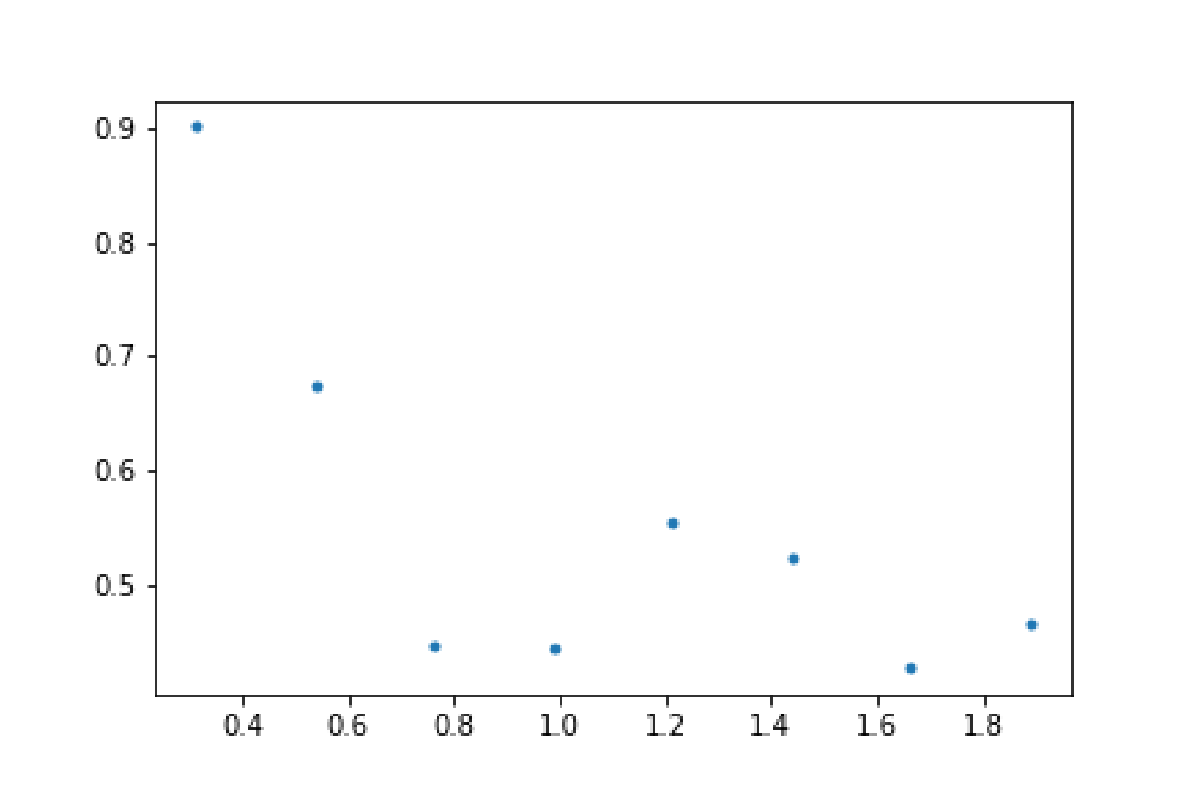
\rho \sim \frac{N_{CC}\rho_{CC} + N^*_{CS}\rho^*_{CS} + N_{CS}\rho_{CS} + N^*_{SS}\rho^*_{SS} + N_{SS}\rho_{SS}}{N_{CC} + N^*_{CS} + N_{CS} + N^*_{SS} + N_{SS}} \qquad \mathbf{2.0}

Final PDF is given in the following table (0.5 for each value):

	$r$	$\rho$
1	0.3125	0.900
2	0.5375	0.674
3	0.7625	0.450
4	0.9875	0.445
5	1.2125	0.556
6	1.4375	0.524
7	1.6625	0.428
8	1.8875	0.466

Note: The constant of normalisation in this case turns out to be 1.00. Hence no need to separately normalise this PDF. 1.0

Most similar to this density is plot E on Figure 1 of question paper. 1.0

Combined original · Solutions - Part 1

Part (a) If we plot given coordinates in XY, XZ and YZ planes we’ll see the following pictures. See Figures 2, 3 and 4 (0.5p for each graph). By observing Figure 2 we can deduce that the group is edge-on and its normal lies in $XY$ plane. $X'$ axis is along line of sight so it can be calculated by normalizing $8.3\hat i+6.2\hat j+1.1\hat k$ . So

\hat x'=0.79667866\hat i+0.59510936\hat j+0.10558392\hat k\qquad (5)

(0.5p) $Z'$ axis lays in $XY$ plane and is perpendicular to $X'$ so it can be calculated by normalizing $\hat x'\times\hat k$

\hat z'=0.59845448\hat i-0.80115681\hat j\qquad (6)

(2p)

Figure 2: XY viewpoint of a cluster from observational site

Figure 3: XZ viewpoint of a cluster from observational site

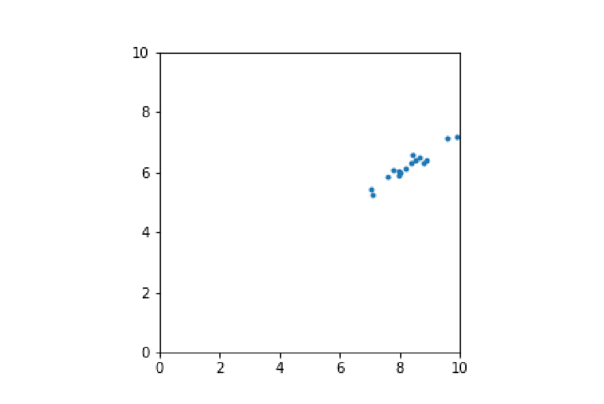
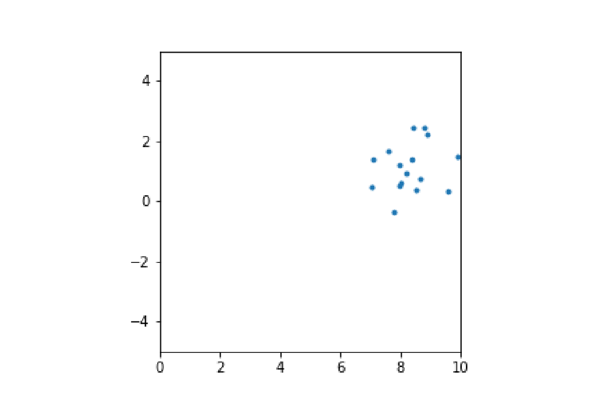
Part (b) One can choose $x'$ as line of sight (found in part(a)) (1p):

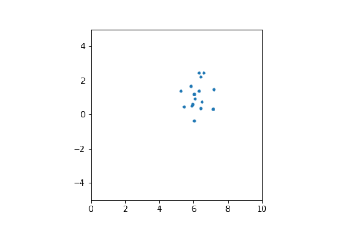
\hat x'=0.79667866\hat i+0.59510936\hat j+0.10558392\hat k\qquad (7)

Figure 4: YZ viewpoint of a cluster from observational site

$z'$ can be chosen as halo disk normal (found in part(a))(1p):

\hat z'=0.59845448\hat i-0.80115681\hat j\qquad (8)

And finally for $y'$ (1p):

\hat y'=\hat x'\times\hat z'=0.08458928\hat i+0.06318717\hat j-0.9944104\hat k\qquad (9)

Part (c) Each coordinate in $X'Y'Z'$ system can be found by following equations

x'=\hat x'\cdot(\vec r-\vec r_c)\qquad (10)

y'=\hat y'\cdot(\vec r-\vec r_c)\qquad (11)

z'=\hat z'\cdot(\vec r-\vec r_c)\qquad (12)

Where $\hat x'$ , $\hat y'$ and $\hat z'$ are unit vectors of local $X'Y'Z'$ system, $\vec r$ is coordinate of a galaxy and $\vec r_c$ is coordinate of the center.

This values are calculated in the following table (0.5p for each correct $x$ , $y'$ , $z'$ tuple):

i	$x-x_c$	$y-y_c$	$z-z_c$	$x'$	$y'$	$z'$
1	0.101124	0.109271	0.294476	0.176684	-0.277372	-0.027025
2	1.582909	0.989392	0.405895	1.892722	-0.207212	0.154641
3	0.582735	0.213285	1.126426	0.710112	-1.057359	0.177866
4	0.144328	0.369381	1.338567	0.476137	-1.295537	-0.209558
5	-0.517770	-0.151687	-1.458202	-0.656729	1.396668	-0.188336
6	0.480059	0.105110	1.362674	0.588881	-1.307808	0.203084
7	-0.309855	-0.319116	-0.568033	-0.496739	0.518483	0.070227
8	0.239541	0.188218	-0.730736	0.225694	0.758807	-0.007438
9	-0.324800	-0.169551	0.116378	-0.347375	-0.153915	-0.058541
10	-1.227659	-0.768684	-0.612379	-1.500158	0.456538	-0.118862
11	-0.263209	-0.234869	-0.485227	-0.400698	0.445410	0.030649
12	0.381200	0.282515	-0.365581	0.433222	0.413634	0.001792
13	-1.185021	-0.941303	0.302593	-1.472310	-0.460620	0.044950
14	1.286640	0.930147	-0.777889	1.496445	0.941150	0.024802
15	-0.106760	-0.095804	-0.184997	-0.161600	0.168879	0.012863
16	-0.686865	-0.352750	0.566244	-0.697350	-0.643470	-0.128449

Part (d) Spherical coordinates can by calculated by following relations:

r=\sqrt{x'^2+y'^2+z'^2}\qquad (13)

\phi=\arctan\frac{y'}{x'}\qquad (14)

and signs of x’ and y’

\theta=\arccos\frac z r\qquad (15)

Calculated values are given in the following table (0.5p for each correct $r$ , $\phi$ , $\theta$ tuple):

i	$x'$	$y'$	$z'$	$r$	$\phi$	$\theta$
1	0.176684	-0.277372	-0.027025	0.329974	5.279566	1.652789
2	1.892722	-0.207212	0.154641	1.910301	6.174141	1.489757
3	0.710112	-1.057359	0.177866	1.286042	5.303793	1.432047
4	0.476137	-1.295537	-0.209558	1.396079	5.064586	1.721471
5	-0.656729	1.396668	-0.188336	1.554814	2.010330	1.692226
6	0.588881	-1.307808	0.203084	1.448581	5.135477	1.430138
7	-0.496739	0.518483	0.070227	0.721461	2.334780	1.473302
8	0.225694	0.758807	-0.007438	0.791695	1.281697	1.580191
9	-0.347375	-0.153915	-0.058541	0.384430	3.558678	1.723672
10	-1.500158	0.456538	-0.118862	1.572587	2.846171	1.646452
11	-0.400698	0.445410	0.030649	0.599906	2.303400	1.519685
12	0.433222	0.413634	0.001792	0.598981	0.762273	1.567805
13	-1.472310	-0.460620	0.044950	1.543336	3.444801	1.541667
14	1.496445	0.941150	0.024802	1.767973	0.561416	1.556768
15	-0.161600	0.168879	0.012863	0.234094	2.334171	1.515821
16	-0.697350	-0.643470	-0.128449	0.957522	3.886829	1.705349

Part (e) Using radii calculated above and number of galaxies for each data (rewritten below) one can calculate number of galaxies in each bin. Range of bin 1 is (0.2, 0.425), bin 2 - (0.425, 0.65) and so on bin 8 - (1.775, 2.0).

i	r	n
1	0.329974	291
2	1.910301	170
3	1.286042	253
4	1.396079	8
5	1.554814	72
6	1.448581	120
7	0.721461	302
8	0.791695	52
9	0.384430	28
10	1.572587	40
11	0.599906	72
12	0.598981	379
13	1.543336	82
14	1.767973	62
15	0.234094	305
16	0.957522	293

Correct values for each bin are: (0.5p for each correct n)

i	Center of the bin	Number of the galaxies
1	0.312500	624
2	0.537500	451
3	0.762500	354
4	0.987500	293
5	1.212500	253
6	1.437500	210
7	1.662500	174
8	1.887500	170

Corresponding histogram is given on Figure 5. (1p)

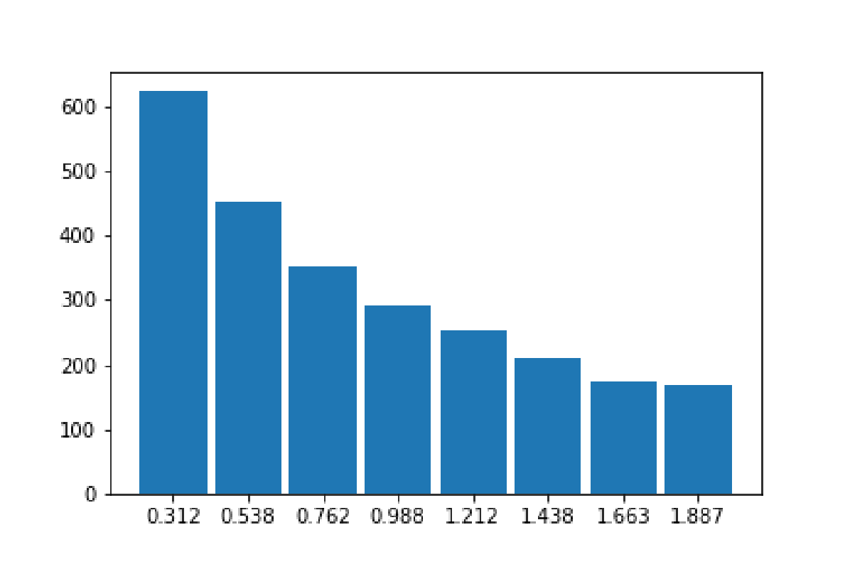
Figure 5: Histogram: Number of galaxies dependence on distance (MPC), with a bin size equal to 0.225 MPC

Histogram data as a table:

In order to get probability density function each value of histogram must be divided by it integral on the whole region. The integral can be approximated by finding total area of the rectangles:

I=\sum_{n=1}^8H(r_i)d=569.025\qquad (16)

Where $d=0.225$ is size of a bin. After dividing each data by $I$ we get (0.25p for each correct probability density):

i	Center of the bin	Number of the galaxies	Probability density
1	0.312500	624	1.096613
2	0.537500	451	0.792584
3	0.762500	354	0.622117
4	0.987500	293	0.514916
5	1.212500	253	0.444620
6	1.437500	210	0.369052
7	1.662500	174	0.305786
8	1.887500	170	0.298757

Plotting this data gives the graph on Figure 6 (1p)

Figure 6: Probability density of center-satellite distances in the same halo

Part (f) Since histogram equation has following form:

H(r)=\frac1{A+B\cdot r}\qquad (17)

We should calculate $1/H(r)$ which gives the following values (0.125 for each correct $1/H$ ):

i	r	H(r)	1/H(r)
1	0.312500	624	0.001603
2	0.537500	451	0.002217
3	0.762500	354	0.002825
4	0.987500	293	0.003413
5	1.212500	253	0.003953
6	1.437500	210	0.004762
7	1.662500	174	0.005747
8	1.887500	170	0.005882

Plotting this data gives Figure 7

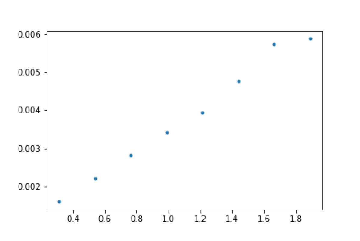
Finding the slope and the intercept of this line (by graph or any other method) gives Following values:

A=0.00065977;\ B=0.00285494\qquad (18)

2.5p for B in range 0.002-0.003 2.5p for A in range 0.0006-0.0008

Combined original · Solutions - Part 2

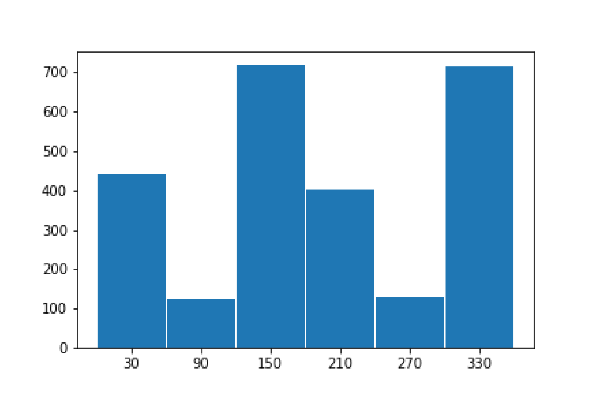
Part (a) We can $\phi$ values from Part 1.c to distribute them in 60 degree bins. In bin 1 we have number of galaxies which fall in (0, 60) degree range, in bin 2 - (60, 120) and so on bin 6 - (300, 360).

Part 1.c data in degrees:

i	Angle	Number of galaxies
1	302.496846	291
2	353.752245	170
3	303.884926	253
4	290.179429	8
5	115.183442	72
6	294.241133	120
7	133.773013	302
8	73.435830	52
9	203.897219	28
10	163.073590	40
11	131.975076	72
12	43.675004	379
13	197.372555	82
14	32.166754	62
15	133.738158	305
16	222.698869	293

We get the following data for the histogram (0.5p for each correct n):

i	Center of the bin	Number of galaxies
1	30	441
2	90	124
3	150	719
4	210	403
5	270	128
6	330	714

Uniform value is total number of galaxies divides by 6 which is 421.5. Square deviation is $241°$ (1p)

Graph is given on Figure 8 (2p)

Figure 8: Histogram: Number of galaxies dependence on $\phi$ angle, with a bin size equal to $60°$

Part (b) A galaxy with the orbital radius $r$ around central mass $M$ has velocity (2p):

v=\sqrt{\frac{GM}{r}}\qquad (19)

This will cause to give the following error in distance along line of sight (2p):

d=\frac v H=\frac1H\sqrt{\frac{GM}{r}}\qquad (20)

Angle difference for galaxies at 90 and 270 degrees will be (2p):

\alpha=\arctan\frac d r=\arctan\frac1H\sqrt{\frac{GM}{r^3}}\qquad (21)

For detailed drawing see Figure 9

Part (c) Galaxies originally in bins of range (60, 120) and (240, 300) might move to (120, 180) and (300, 360) respectively. So we should subtract correction value found in previous task to the galaxies in bins 2 and 5 to see if they move to bins 1 and 4 respectively. (0.25p for each correct corrected angle(

i	Original angle	Corrected angle	Number of galaxies
1	302.494665	276.136451	291
2	353.752069	351.714594	170
3	303.884728	300.199512	253
4	290.178642	290.178642	8
5	115.184577	115.184577	72
6	294.241835	294.241835	120
7	133.776280	125.061576	302
8	73.437747	73.437747	52
9	203.899065	203.899065	28
10	163.073490	160.346665	40
11	131.977481	120.548626	72
12	43.676971	43.676971	379
13	197.372956	197.372956	82
14	32.167948	32.167948	62
15	133.743596	94.077612	305
16	222.694636	222.694636	293

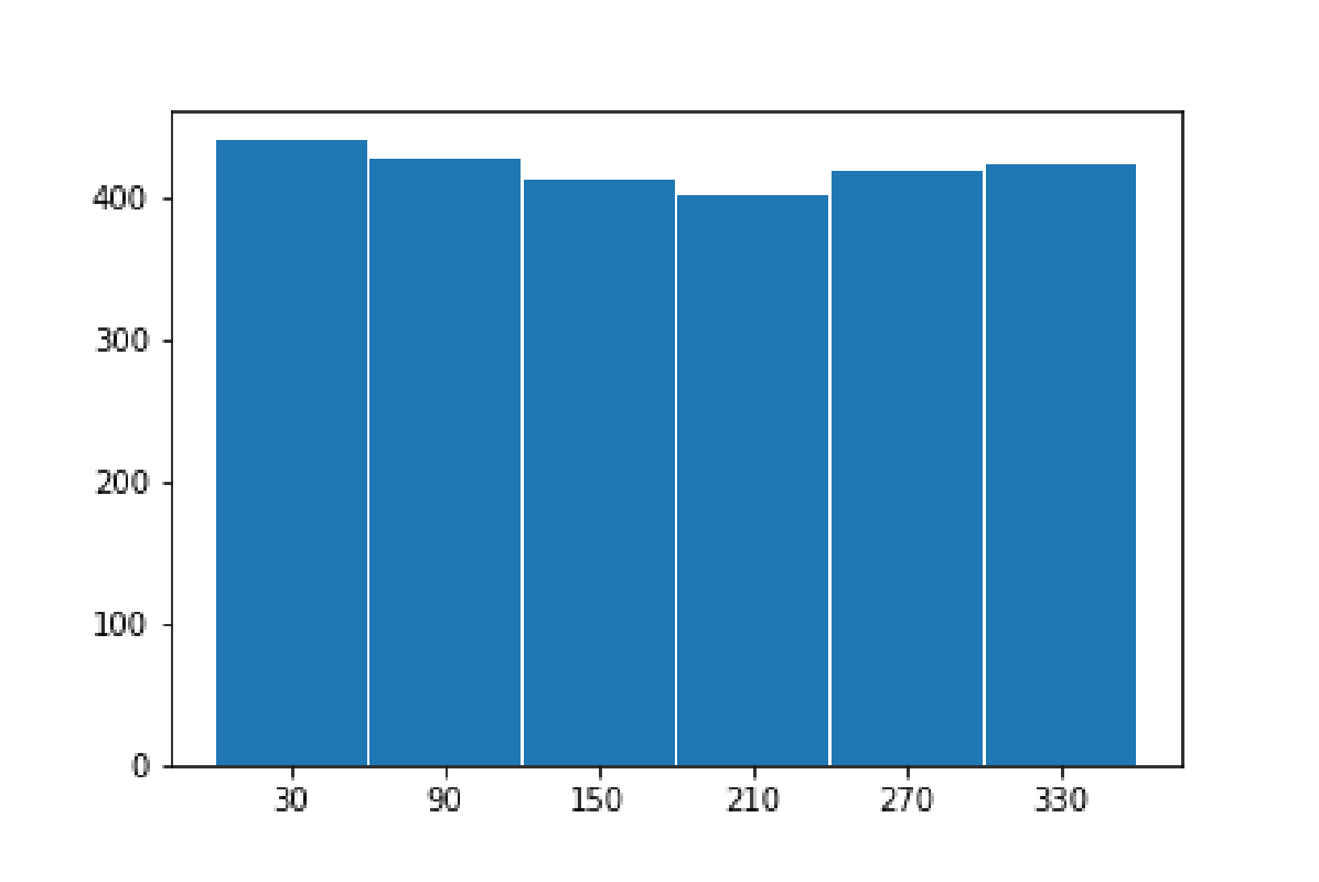
New corrected distribution looks like this (0.3p for each correct n):

i	Center of the bin	Number of galaxies
1	30	441
2	90	429
3	150	414
4	210	403
5	270	419
6	330	423

In this case square deviation equals to $12°$

(1p) And relevant graph is given on Figure 10 (1.2p)

Figure 10: Histogram: Corrected Number of galaxies dependence on $\phi$ angle, with a bin size equal to $60°$

Combined original · Solutions - Part 3

Part (a) With simple combinatorics one can get (0.6p for each correct N):

N_{CC}=N_C(N_C-1)=249500\qquad (22)

N^*_{CS}=N_CN_S=500000\qquad (23)

N_{CS}=N_C(N_C-1)N_S=249500000\qquad (24)

N^*_{SS}=N_CN_S(N_S-1)=499500000\qquad (25)

N_{SS}=N_CN_S(N_C-1)N_S=249500000000\qquad (26)

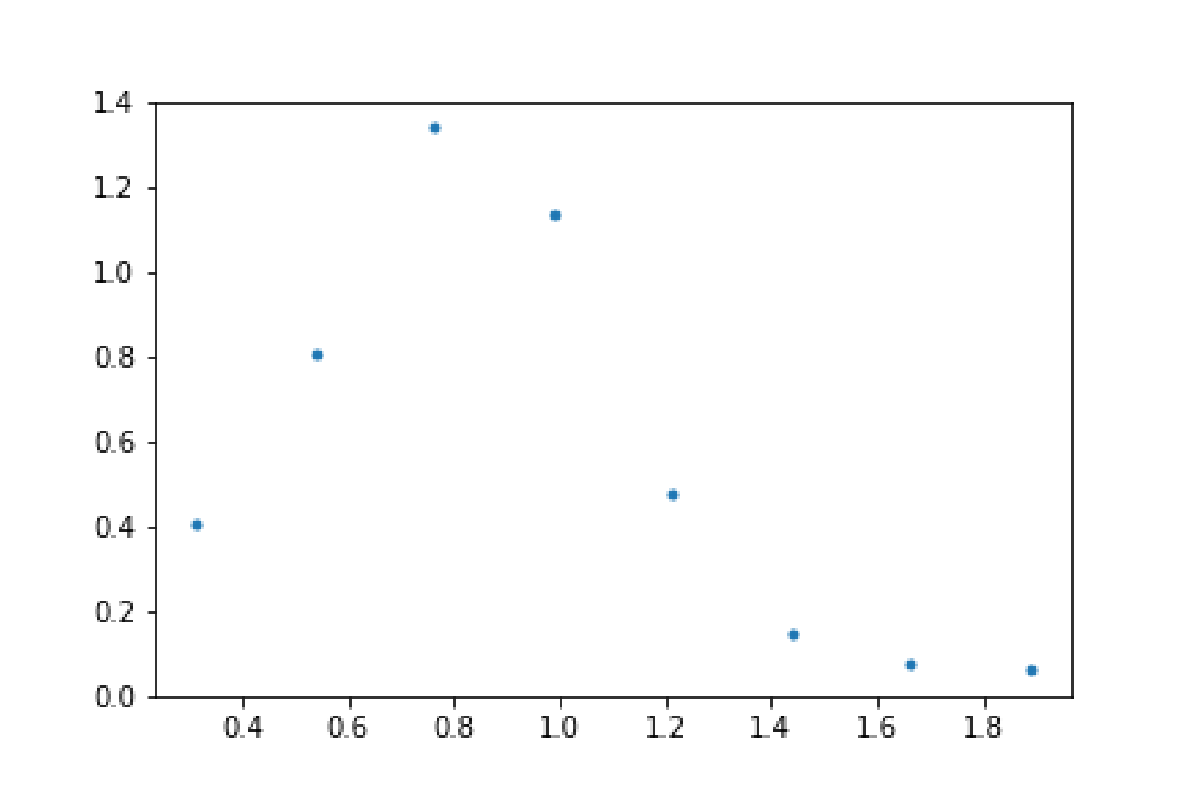
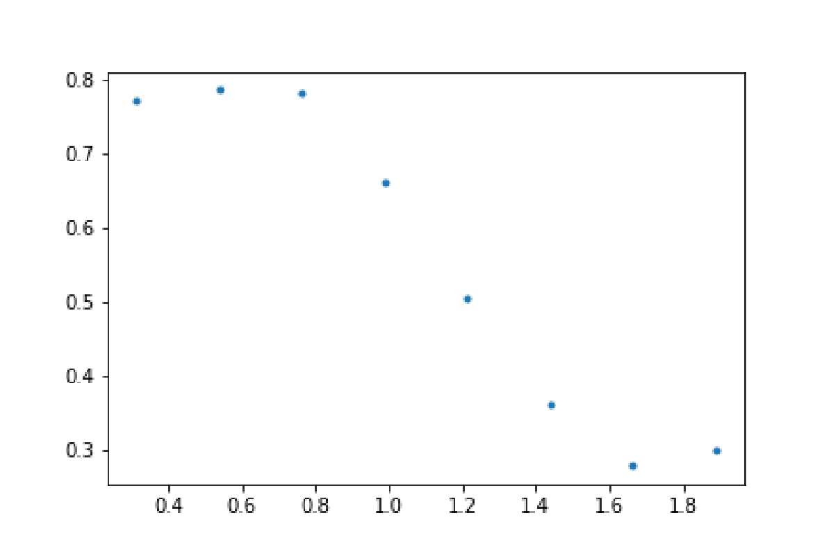
Part (b) We can calculate all probability densities using center-center and center-satellite densities. Non-normalized values (with $c_1=c_2=c_3=1$ ) are calculated in the following table (0.5p for each correct tuple):

i	r	$\rho^*_{CS}$	$\rho_{CC}$	$\rho^*_{SS}$	$\rho_{SS}$	$\rho_{CS}$
1	0.312500	1.096613	0.406141	0.375800	17.365137	0.975747
2	0.537500	0.792584	0.807863	0.337652	12.992898	0.994072
3	0.762500	0.622117	1.340510	0.295110	8.653487	0.988565
4	0.987500	0.514916	1.134011	0.261824	8.568351	0.837480
5	1.212500	0.444620	0.478630	0.239696	10.729180	0.638199
6	1.437500	0.369052	0.143154	0.195787	10.112507	0.458355
7	1.662500	0.305786	0.073165	0.155452	8.262279	0.352612
8	1.887500	0.298757	0.060971	0.168470	8.998531	0.379962

For normalization (same way as in Part 1.d) we get $c_1=2.18592$ ; $c_2=0.79304$ ; $c_3=0.0516$ . Multiplying relevant densities by this values gives (0.5p for each correct normalized tuple):

i	r	$\rho^*_{SS}$	$\rho_{SS}$	$\rho_{CS}$
1	0.312500	0.822854	0.900750	0.770962
2	0.537500	0.739325	0.673957	0.785441
3	0.762500	0.646175	0.448866	0.781089
4	0.987500	0.573292	0.444450	0.661713
5	1.212500	0.524839	0.556535	0.504257
6	1.437500	0.428697	0.524548	0.362158
7	1.662500	0.340380	0.428574	0.278607
8	1.887500	0.368883	0.466764	0.300217

Plots are given on Figures 11 - 14 (0.5p for each plot).

Part (c) Total probability density is weighted sum of all densities (4p):

\rho\sim\frac{N_{CC}\rho_{CC}+N^*_{CS}\rho^*_{CS}+N_{CS}\rho_{CS}+N^*_{SS}\rho^*_{SS}+N_{SS}\rho_{SS}}{N_{CC}+N^*_{CS}+N_{CS}+N^*_{SS}+N_{SS}}\qquad (27)

Calculated values and normalized densities are given in the following table:

Figure 11: Probability density of center-center distances in for different halos

Figure 12: Probability density of center-satellite distances in the different halos

Figure 13: Probability density of satellite-satellite distances in the different halos

Figure 14: Probability density of satellite-satellite distances in the same halo

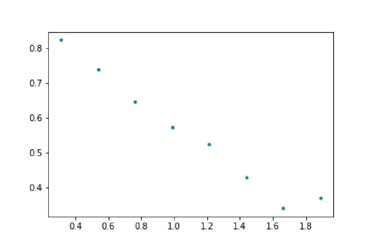
i	r	Calculated $\rho$	Normalized $\rho$
1	0.312500	0.004212	0.843662
2	0.537500	0.003606	0.722433
3	0.762500	0.002967	0.594357
4	0.987500	0.002693	0.539524
5	1.212500	0.002663	0.533361
6	1.437500	0.002265	0.453652
7	1.662500	0.001813	0.363239
8	1.887500	0.001968	0.394216

And final plot looks like this (Figure 15) (2p)

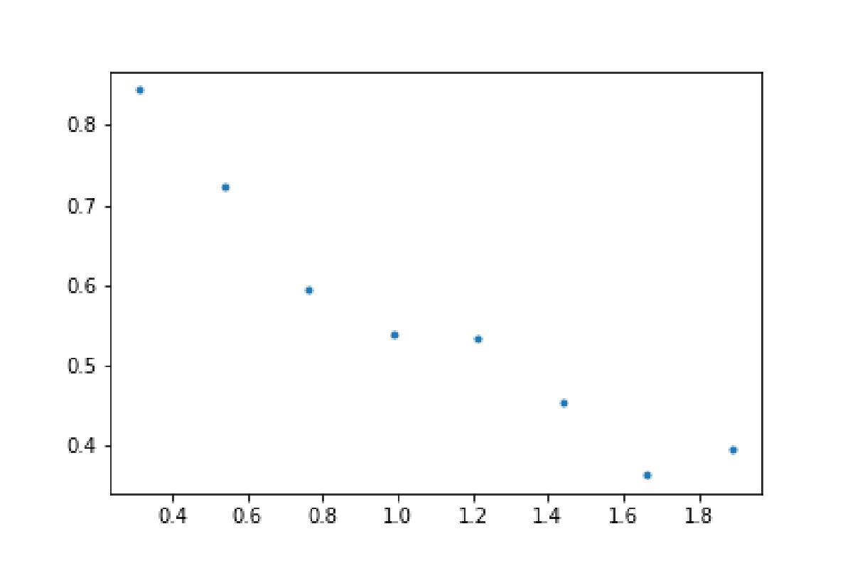
Most similar to this density is plot E on Figure 1 (1p).

Оригинал в Архива: IOAA-Data.pdf · официални решения: Data_Solution.pdf · допълнителни данни: Data Analysis Problems & Solutions.pdf