IOAA 2025, Анализ на данни — Задача 2. D02 · Predicting arrival times of coronal mass ejections on Earth
18th IOAA, Mumbai 2025 — Data Analysis Examination · 60 т.
Внимание: Бележка към темата
The obtained Summary Answersheet contains D02 only. Referenced D01 response forms were unavailable; all D01 data graphs printed in the question and solution booklets are retained.
Условие
The Sun occasionally releases magnetized plasma, termed coronal mass ejections (CMEs), that originate from the surface of the Sun and propagate outwards. Accurate prediction of their arrival times at Earth is crucial for understanding and mitigating their potential effects on satellites orbiting the Earth. In this problem, we aim to predict the arrival times of CMEs by developing an empirical model, using the data of 10 CMEs. Throughout this problem, the distance between the Sun’s surface and Earth is taken to be . Further, assume that the Sun is not rotating.
Due to electromagnetic, gravitational and drag forces, CMEs experience a variable acceleration throughout their propagation. In the first two parts of this problem, we assume that the region between the Sun and the Earth is vacuum.
CMEs through vacuum
(D02.1) The initial velocity, , at the solar surface , the final velocity, , upon reaching Earth, and the time to arrive at Earth after leaving the surface of the Sun (in hours), , are given for 10 CMEs in the following table.
| CME Name | () | () | () |
|---|---|---|---|
| CME-A | 804 | 470 | 74.5 |
| CME-B | 247 | 360 | 127.5 |
| CME-C | 523 | 396 | 103.5 |
| CME-D | 830 | 415 | 71.0 |
| CME-E | 665 | 400 | 104.5 |
| CME-F | 347 | 350 | 101.5 |
| CME-G | 446 | 375 | 99.5 |
| CME-H | 155 | 360 | 97.0 |
| CME-I | 1016 | 515 | 67.0 |
| CME-J | 683 | 410 | 54.0 |
(D02.1a) [3 marks] Calculate the average acceleration, , for each CME in .
(D02.1b) [15 marks] We assume an empirical model for the acceleration, , of a CME, which depends on its initial velocity, , as where, is expressed in , is expressed in and .
Determine the constants and and their associated uncertainties using an appropriate graph (mark your graph as “D02.1b”).
(D02.1c) [4 marks] For each CME, tabulate in . Hence calculate the root-mean-square (rms) deviation of acceleration, , between the calculated accelerations, , and the model values, .
(D02.2) We consider two other CMEs: CME-1 and CME-2, with initial velocities, and , respectively.
(D02.2a) [4 marks] Using the empirical model obtained in (D02.1b), calculate the predicted arrival times at Earth, and (in hours), for CME-1 and CME-2, respectively.
(D02.2b) [2 marks] The observed arrival times at Earth of CME-1 and CME-2 are and , respectively. The empirical model is considered to be VALID for a particular CME if its predicted arrival time is within 20% of its observed arrival time; otherwise, it is NOT VALID. Indicate the validity of the model for each CME by ticking (✓) the appropriate box in the Summary Answersheet.
CMEs in presence of solar wind
In reality, the space between the Sun and the Earth is permeated with the solar wind, which exerts a drag force on CMEs. This drag force can either decelerate or accelerate a CME, depending on the CME’s velocity relative to that of the solar wind. To account for the solar wind’s influence, we will use a “drag-only” model for distances , where is the distance beyond which the drag force becomes the dominant force affecting the CME’s motion.
The distance from the surface of the Sun as determined from the “drag-only” model, , and velocity, , of a CME in this model is given by
where, , is the constant speed of the solar wind, and are the distance and velocity, respectively, at time , and is the sign factor. if ; if .
(D02.3) The tables below show the observed radial distance from the surface of the Sun, (measured in ), as a function of time, (in hours), for two CMEs: CME-3 and CME-4. The last data point in each table (D5 and P8, respectively) corresponds to the arrival time of the respective CME at Earth. For this part, assume .
CME-3
| Data point | (in h) | (in ) |
|---|---|---|
| D1 | 0.200 | 6.36 |
| D2 | 0.480 | 7.99 |
| D3 | 1.22 | 11.99 |
| D4 | 1.49 | 13.51 |
| D5 | 58.05 | 214 |
CME-4
| Data point | (in h) | (in ) |
|---|---|---|
| P1 | 1.00 | 4.00 |
| P2 | 3.00 | 6.00 |
| P3 | 4.00 | 9.00 |
| P4 | 5.00 | 11.0 |
| P5 | 21.0 | 43.0 |
| P6 | 50.0 | 100 |
| P7 | 85.0 | 170 |
| P8 | 111 | 214 |
We shall evaluate if the “drag-only” model satisfactorily predicts the arrival times of these CMEs. To use this model an appropriate choice of , and corresponding and needs to be made.
(D02.3a) [6 marks] For CME-3, take the following two cases:
(C1) is taken as the midpoint of the interval D1 – D2
(C2) is taken as the midpoint of the interval D3 – D4
Assume the velocity remains constant in each specific interval D1–D2 and D3–D4, but may differ between the two intervals.
Using , , and , calculate the difference between the observed and the predicted radial distance, in units of at , for each of the two cases.
(D02.3b) [4 marks] Evaluate at points, P5, P6, P7, and P8 between the Sun and the Earth for CME-4 for the following two cases adopting the procedure similar to (D02.3a):
(C3) is taken as the midpoint of the interval P1 – P2
(C4) is taken as the midpoint of the interval P3 – P4
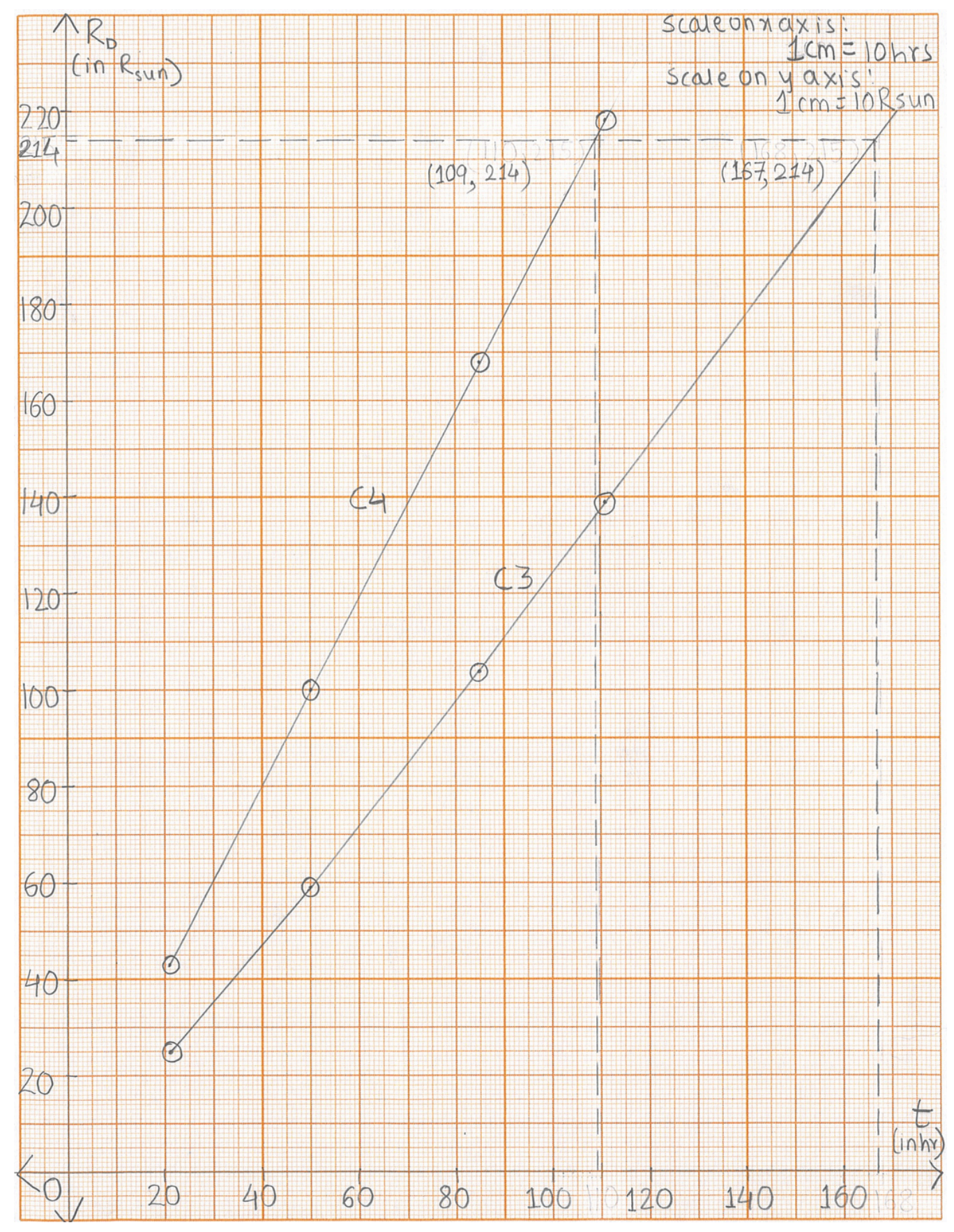
(D02.3c) [10 marks] Plot (in ) vs (in hours) for the two cases, C3 and C4, for CME-4 at points, P5, P6, P7, and P8 (mark your graph as “D02.3c”). On the same graph, draw smooth curves of for the above mentioned two cases. For this part, take the range of axis from 0 to 180 h.
(D02.3d) [4 marks] Using the graph, estimate the absolute difference, between the actual arrival time of CME-4 at the Earth and its time of arrival predicted by the drag-only model, for each of the cases C3 and C4.
(D02.3e) [1 mark] Indicate whether the following statement is TRUE or FALSE by ticking (✓) the appropriate box in the Summary Answersheet (no written justification needed):
“The drag forces exerted by the solar wind on CMEs become dominant for CME-3 at an earlier time compared to CME-4.”
(D02.4) [7 marks] Consider drag as the dominant force acting on 10 CMEs in part D02.1. Assume that the “drag-only” model is applicable from the surface of the Sun and beyond, for all CMEs. Estimate and tabulate the solar wind speed in for each CME. Further, estimate the average solar wind speed for all 10 CMEs.
Решение
(D02.1a) Solution:
Average acceleration (in ) is given by the following relation,
| CME Name | () | () | (h) | () |
|---|---|---|---|---|
| CME-A | 804 | 470 | 74.5 | −1.25 |
| CME-B | 247 | 360 | 127.5 | 0.246 |
| CME-C | 523 | 396 | 103.5 | −0.341 |
| CME-D | 830 | 415 | 71.0 | −1.62 |
| CME-E | 665 | 400 | 104.5 | −0.704 |
| CME-F | 347 | 350 | 101.5 | 0.00821 |
| CME-G | 446 | 375 | 99.5 | −0.198 |
| CME-H | 155 | 360 | 97.0 | 0.587 |
| CME-I | 1016 | 515 | 67.0 | −2.08 |
| CME-J | 683 | 410 | 54.0 | −1.40 |
(D02.1b) Solution:
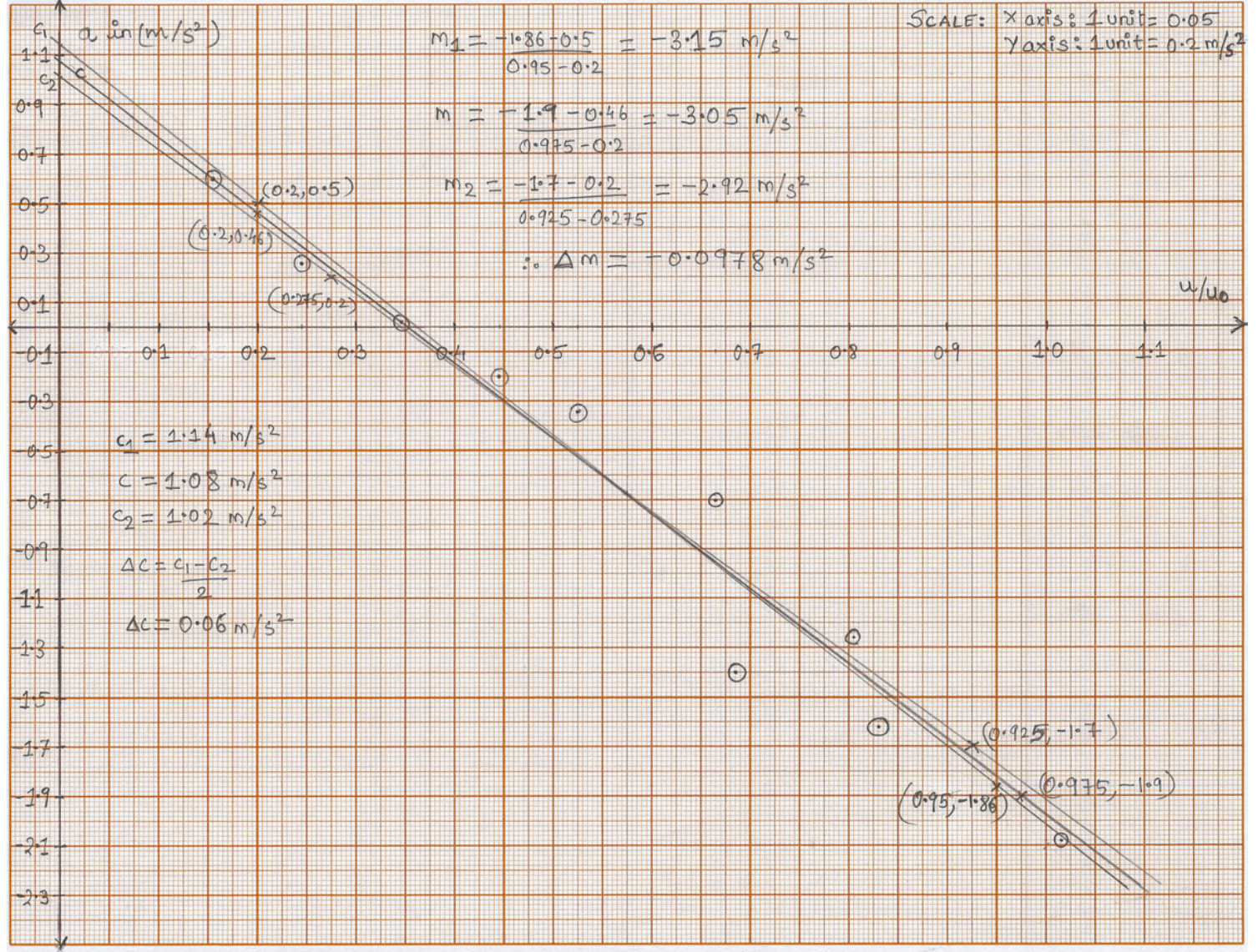
Thus, the expression obtained by fitting a straight line to vs is
(D02.1c) Solution:
| CME Name | () |
|---|---|
| CME-A | −1.37 |
| CME-B | 0.327 |
| CME-C | −0.515 |
| CME-D | −1.45 |
| CME-E | −0.948 |
| CME-F | 0.0217 |
| CME-G | −0.280 |
| CME-H | 0.607 |
| CME-I | −2.02 |
| CME-J | −1.00 |
The root mean square (rms) deviation of acceleration is given by
Using this expression we get,
(D02.2a) Solution:
The time of arrival of a CME at the Earth, , can be calculated from the following relation.
However, this would yield two solutions for , only one of which will be for a positive final velocity (acceptable), and the other for a negative final velocity (not acceptable). Since acceleration is constant, the final velocity at Earth at a distance is given by
Using this velocity, we get the arrival time as
Using the given value of , and the obtained values of and , we get
For CME-1:
which gives
For CME-2:
which gives
(D02.2b) Solution:
The arrival time for CME-1 is ,
therefore the percentage error in the arrival time of CME-1 is,
Similarly, the arrival time for CME-2 is ,
hence the percentage error is arrival time for CME-2 is,
| VALID | NOT VALID | |
|---|---|---|
| CME-1 | ✓ | |
| CME-2 | ✓ |
(D02.3a) Solution:
Inserting, , , , and in the given expression
we get
Case C1:
we get, at .
Thus, .
Case C2:
Using the expression above, at .
Thus, .
(D02.3b) Solution:
Case C3:
Case C4:
| Data Point | (h) | C3: () | C4: () |
|---|---|---|---|
| P5 | 21.0 | 25.1 | 42.8 |
| P6 | 50.0 | 59.1 | 99.9 |
| P7 | 85.0 | 104 | 168 |
| P8 | 111 | 139 | 218 |
(D02.3c) Solution:
The plot below shows the data points of CME-4 and smooth variation of extrapolated up to .
(D02.3d) Solution:
The arrival time of CME at Earth () can be obtained by estimating the point of intersection between and two smooth curves.
The points of intersection are and for the cases C3 and C4, respectively.
Thus, absolute time differences are:
and
.
(D02.3e) Solution:
The statement is TRUE.
In the scenario of CME-3, the “drag-only” model predicts the arrival distance accurately when is computed using the initial velocity, and initial distance, at and beyond.
While for CME-4, the “drag-only” model start accurately predicting the arrival times of CME-4 when is calculated using and at after the launch of the CME.
(D02.4) Solution:
Taking, if , else the above expression is quadratic equation, thus, we get two values of . If , choose the solution with . If , choose the solution with .
Calculating using the above conditions for all ten CMEs.
| CME Name | () | () | (h) | () |
|---|---|---|---|---|
| CME-A | 804 | 470 | 74.5 | 337 |
| CME-B | 247 | 360 | 127.5 | 428 |
| CME-C | 523 | 396 | 103.5 | 314 |
| CME-D | 830 | 415 | 71.0 | 270 |
| CME-E | 665 | 400 | 104.5 | 303 |
| CME-F | 347 | 350 | 101.5 | 369 |
| CME-G | 446 | 375 | 99.5 | 305 |
| CME-H | 155 | 360 | 97.0 | 457 |
| CME-I | 1016 | 515 | 67.0 | 357 |
| CME-J | 683 | 410 | 54.0 | 248 |
Taking the average of the solar wind speed, , for each case, we get
D02 Summary Answersheet — SA-1
Summary Answersheet — FRONT
Contestant Code: ______ – ______
Q. No. D02 · Page No. SA-1
Final answers
(D02.1a) Marks (3.0)
| CME Name | () | () | (h) | |||
|---|---|---|---|---|---|---|
| CME-A | 804 | 470 | 74.5 | |||
| CME-B | 247 | 360 | 127.5 | |||
| CME-C | 523 | 396 | 103.5 | |||
| CME-D | 830 | 415 | 71.0 | |||
| CME-E | 665 | 400 | 104.5 | |||
| CME-F | 347 | 350 | 101.5 | |||
| CME-G | 446 | 375 | 99.5 | |||
| CME-H | 155 | 360 | 97.0 | |||
| CME-I | 1016 | 515 | 67.0 | |||
| CME-J | 683 | 410 | 54.0 |
(D02.1b) Marks (15.0)
Graph number: D02.1b
______
______
D02 Summary Answersheet — SA-2
Summary Answersheet — BACK
Contestant Code: ______ – ______
Q. No. D02 · Page No. SA-2
Final answers
(D02.1c) Marks (4.0)
| CME Name | () |
|---|---|
| CME-A | |
| CME-B | |
| CME-C | |
| CME-D | |
| CME-E | |
| CME-F | |
| CME-G | |
| CME-H | |
| CME-I | |
| CME-J |
______
(D02.2a) Marks (4.0)
______ h
______ h
(D02.2b) Marks (2.0)
| VALID | NOT VALID | |
|---|---|---|
| CME-1 | ||
| CME-2 |
D02 Summary Answersheet — SA-3
Summary Answersheet — FRONT
Contestant Code: ______ – ______
Q. No. D02 · Page No. SA-3
Final answers
(D02.3a) Marks (6.0)
C1:
______
C2:
______
(D02.3b) Marks (4.0)
| Data Point | (h) | C3: () | C4: () |
|---|---|---|---|
| P5 | 21.0 | ||
| P6 | 50.0 | ||
| P7 | 85.0 | ||
| P8 | 111 |
(D02.3c) Marks (10.0)
Graph number: D02.3c
D02 Summary Answersheet — SA-4
Summary Answersheet — BACK
Contestant Code: ______ – ______
Q. No. D02 · Page No. SA-4
Final answers
(D02.3d) Marks (4.0)
C3: ______
C4: ______
(D02.3e) Marks (1.0)
TRUE □ FALSE □
(D02.4) Marks (7.0)
| CME Name | () | () | (h) | () |
|---|---|---|---|---|
| CME-A | 804 | 470 | 74.5 | |
| CME-B | 247 | 360 | 127.5 | |
| CME-C | 523 | 396 | 103.5 | |
| CME-D | 830 | 415 | 71.0 | |
| CME-E | 665 | 400 | 104.5 | |
| CME-F | 347 | 350 | 101.5 | |
| CME-G | 446 | 375 | 99.5 | |
| CME-H | 155 | 360 | 97.0 | |
| CME-I | 1016 | 515 | 67.0 | |
| CME-J | 683 | 410 | 54.0 |
______
Total: ______
End of Summary Answersheet
Оригинал в Архива: Data-Analysis-Questions.pdf · официални решения: Data-Analysis-Solutions.pdf · допълнителни данни: Data-Analysis-Summary-Answersheet.pdf