Съдържание
УсловиеEquipment and instrument guideOscilloscope. Oscilloscope is an electronic device designed to visualize electric signal applied to its input. An oscilloscope plots on its display a set of points separated by a small time interval related to the oscilloscope sampling rate. At the automatic sweep mode the vertical coordinate of a point is proportional to a current magnitude of the signal (appropriately scaled) while the horizontal coordinate is equal to the ratio of the number of time intervals passed to the sampling rate. In so doing, the oscilloscope plots on the display time dependence of the signal. An oscilloscope inputs are usually referred to as «channels». In this experiment a two-channel oscilloscope is used. It allows one to observe simultaneously time dependence of two signals applied to its channels. Option of continuous signal recording is not provided by this oscilloscope, it displays only a signal sampled over a limited time interval. In other words time dependence of the signal is plotted only during this time interval. Its duration is set by a timebase control. When the timebase is set to maximum the oscilloscope shows the plot of maximum duration, however the sampling rate in this case is also the lowest. It will be not possible to display properly a signal with a typical variation rate comparable to the sampling rate or even exceeding it. Therefore the timebase must be properly set in order to observe the signal in detail. For instance, when a repetitive signal is being studied several periods should be displayed. The oscilloscope trigger menu is used to set the moment when the oscilloscope starts plotting the signal sample and the period of its display. For choosing the language use the page 1/4 of the menu «УТИЛИТЫ» (4 on Fig.3). The synchronization menu allows to regulate the time of initiation of the signal processing and the periodicity of its display. In the synchronization menu (denoted «СИНХР» 1 Ошибка! Источник ссылки не найден..) press the button «МЕНЮ СИНХР» (2 on Fig.1) to adjust the synchronization of the oscilloscope. By default the menu is set as follows: menu «Type» - «Edge» (3 on Ошибка! Источник ссылки не найден..),menu «Source» - «CH1» (4 on Ошибка! Источник ссылки не найден..), menu «Slope» - «↑» (5 on Ошибка! Источник ссылки не найден..), menu «Mode» - «Auto» (6 on Ошибка! Источник ссылки не найден..). If the menu on your equipment is set differently, return it to the default settings using grey buttons at the right side of the screen. Also there in the a menu «СИНХР» you can change the level of the signal by rotating the button «УРОВЕНЬ» (7 on Ошибка! Источник ссылки не найден..)). the rotation of that button may move the trigger mark on the left side of the screen (8 on Ошибка! Источник ссылки не найден..)). To set the synchronization you have to set the «УРОВЕНЬ» so that it will be in the range of the signal of the first channel of the oscilloscope. To regulate the scale of the displacement of signal on vertical axes use the big turning buttons in the menu «ВЕРТИК» (10 on Ошибка! Источник ссылки не найден..). To displace the signals vertically use for each signal the turning buttons «СМЕЩЕНИЕ» (11 onОшибка! Источник ссылки не найден..). The scale and displacements on horizontal axes are regulated similarly by the buttons in the menu «ГОРИЗОНТ» (12 on Ошибка! Источник ссылки не найден..).GeneratorUltrasound receiver/transducerAmplifierLuxmeter (light intensity) meterEquipment listPrefacePart 1. Sound waves. Measurement of speed of sound by phase method.Part 2. Measurement of speed of sound by pulse method. Anisotropy of speed of sound in wood.Part 3. Electromagnetic waves. Study of unpolarised and linearly polarised light.Part 4. Study of elliptically polarised light.РешениеIOM 2016, Експеримент — Задача 1. Anisotropy
The 1st International Olympiad of Metropolises — Physics experiment · 6 септември 2016 г. · 100 т.
Внимание: Бележка към темата
The complete retained English question packet, instrument manual and matching archived key are transcribed. Printed broken Word references, interrupted manual sentence, repeated figure numbers and key formula/unit/data/rubric discrepancies remain literal with separately labelled source notes. The separate blank answer sheet and polar coordinate paper requested in the questions are not retained in this source set; the full key includes completed data, plots and grading.
Native packet heading
The 1st International Olympiad of Metropolises.
Physics. 6 September 2016
The original repeats this heading on every question page. The first six PDF pages are the equipment photograph and instrument guide; the following ten pages are the connected experiment. The native key ends with Total: 100.
Условие
Equipment and instrument guide
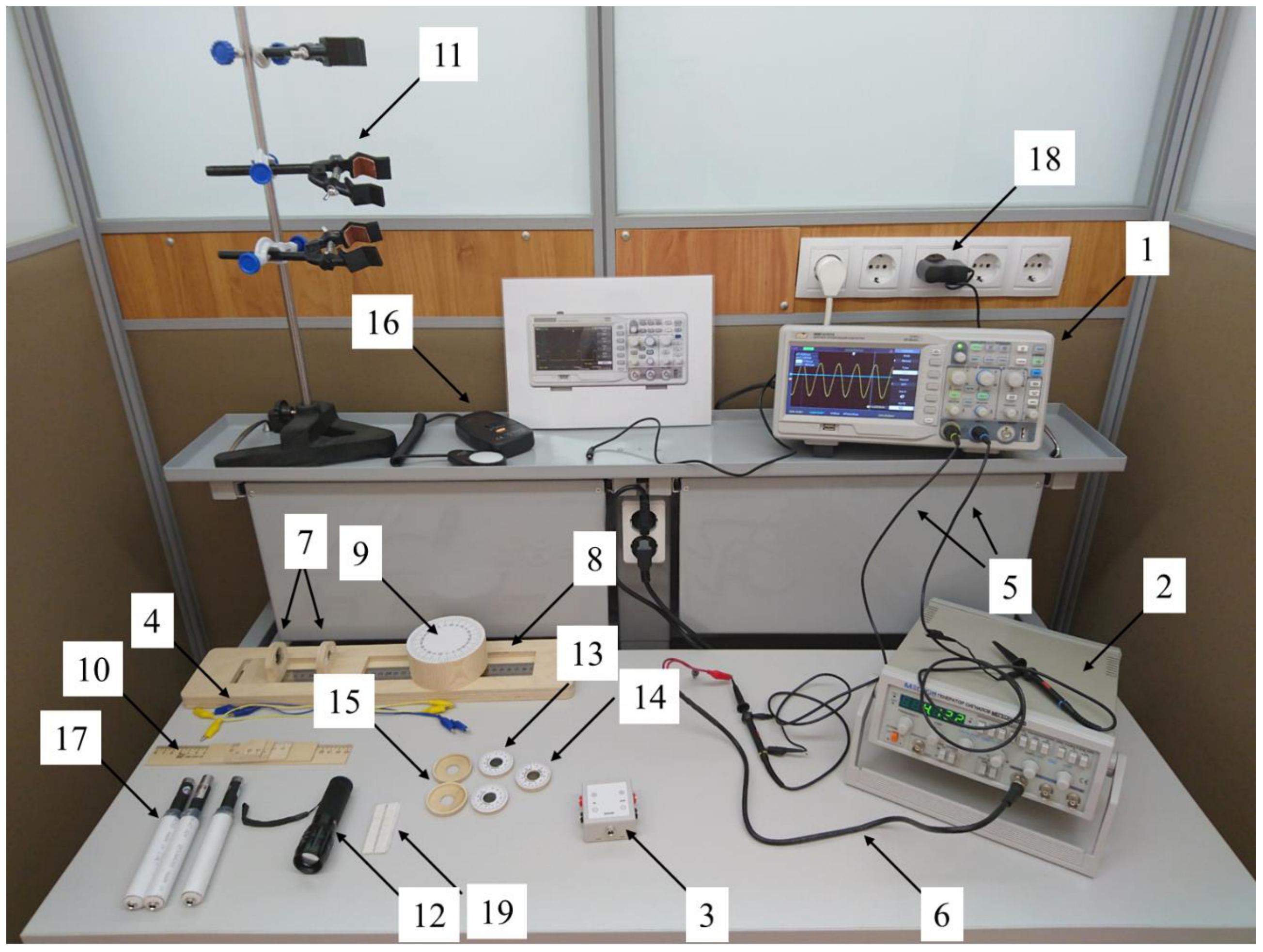
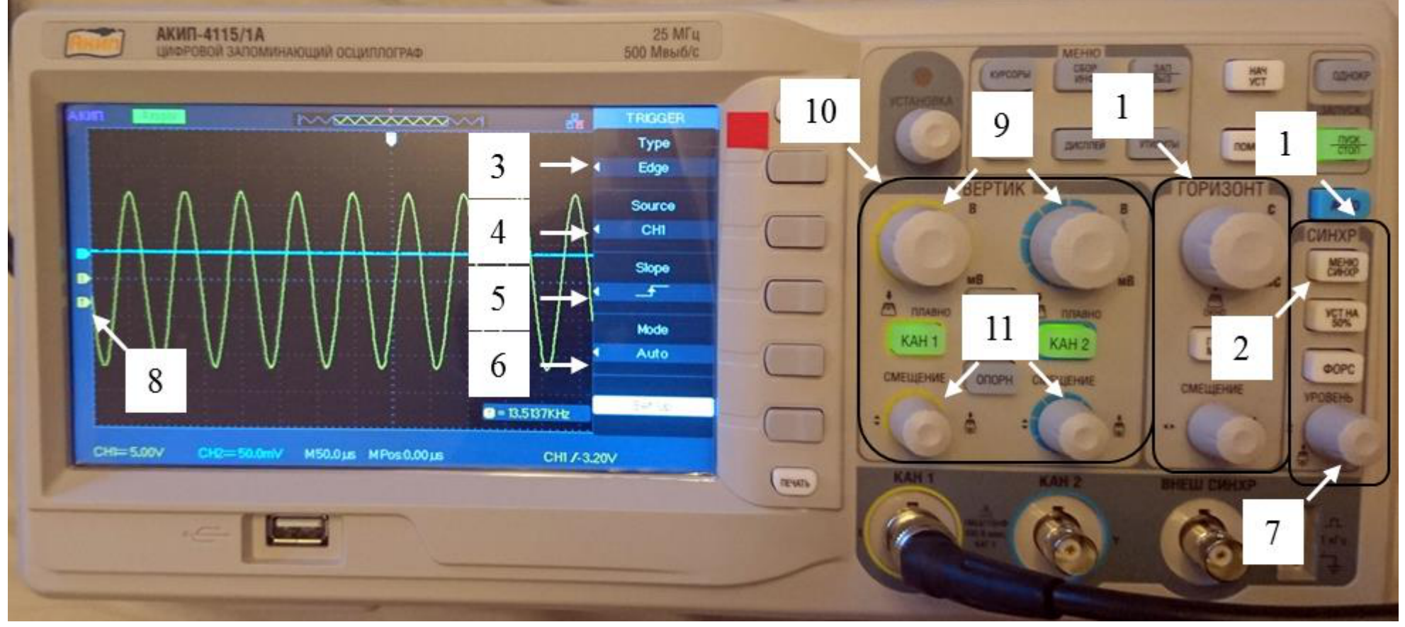
Oscilloscope. Oscilloscope is an electronic device designed to visualize electric signal applied to its input. An oscilloscope plots on its display a set of points separated by a small time interval related to the oscilloscope sampling rate. At the automatic sweep mode the vertical coordinate of a point is proportional to a current magnitude of the signal (appropriately scaled) while the horizontal coordinate is equal to the ratio of the number of time intervals passed to the sampling rate. In so doing, the oscilloscope plots on the display time dependence of the signal. An oscilloscope inputs are usually referred to as «channels». In this experiment a two-channel oscilloscope is used. It allows one to observe simultaneously time dependence of two signals applied to its channels. Option of continuous signal recording is not provided by this oscilloscope, it displays only a signal sampled over a limited time interval. In other words time dependence of the signal is plotted only during this time interval. Its duration is set by a timebase control. When the timebase is set to maximum the oscilloscope shows the plot of maximum duration, however the sampling rate in this case is also the lowest. It will be not possible to display properly a signal with a typical variation rate comparable to the sampling rate or even exceeding it. Therefore the timebase must be properly set in order to observe the signal in detail. For instance, when a repetitive signal is being studied several periods should be displayed. The oscilloscope trigger menu is used to set the moment when the oscilloscope starts plotting the signal sample and the period of its display. For choosing the language use the page 1/4 of the menu «УТИЛИТЫ» (4 on Fig.3). The synchronization menu allows to regulate the time of initiation of the signal processing and the periodicity of its display. In the synchronization menu (denoted «СИНХР» 1 Ошибка! Источник ссылки не найден..) press the button «МЕНЮ СИНХР» (2 on Fig.1) to adjust the synchronization of the oscilloscope. By default the menu is set as follows: menu «Type» - «Edge» (3 on Ошибка! Источник ссылки не найден..),menu «Source» - «CH1» (4 on Ошибка! Источник ссылки не найден..), menu «Slope» - «↑» (5 on Ошибка! Источник ссылки не найден..), menu «Mode» - «Auto» (6 on Ошибка! Источник ссылки не найден..). If the menu on your equipment is set differently, return it to the default settings using grey buttons at the right side of the screen. Also there in the a menu «СИНХР» you can change the level of the signal by rotating the button «УРОВЕНЬ» (7 on Ошибка! Источник ссылки не найден..)). the rotation of that button may move the trigger mark on the left side of the screen (8 on Ошибка! Источник ссылки не найден..)). To set the synchronization you have to set the «УРОВЕНЬ» so that it will be in the range of the signal of the first channel of the oscilloscope. To regulate the scale of the displacement of signal on vertical axes use the big turning buttons in the menu «ВЕРТИК» (10 on Ошибка! Источник ссылки не найден..). To displace the signals vertically use for each signal the turning buttons «СМЕЩЕНИЕ» (11 onОшибка! Источник ссылки не найден..). The scale and displacements on horizontal axes are regulated similarly by the buttons in the menu «ГОРИЗОНТ» (12 on Ошибка! Источник ссылки не найден..).
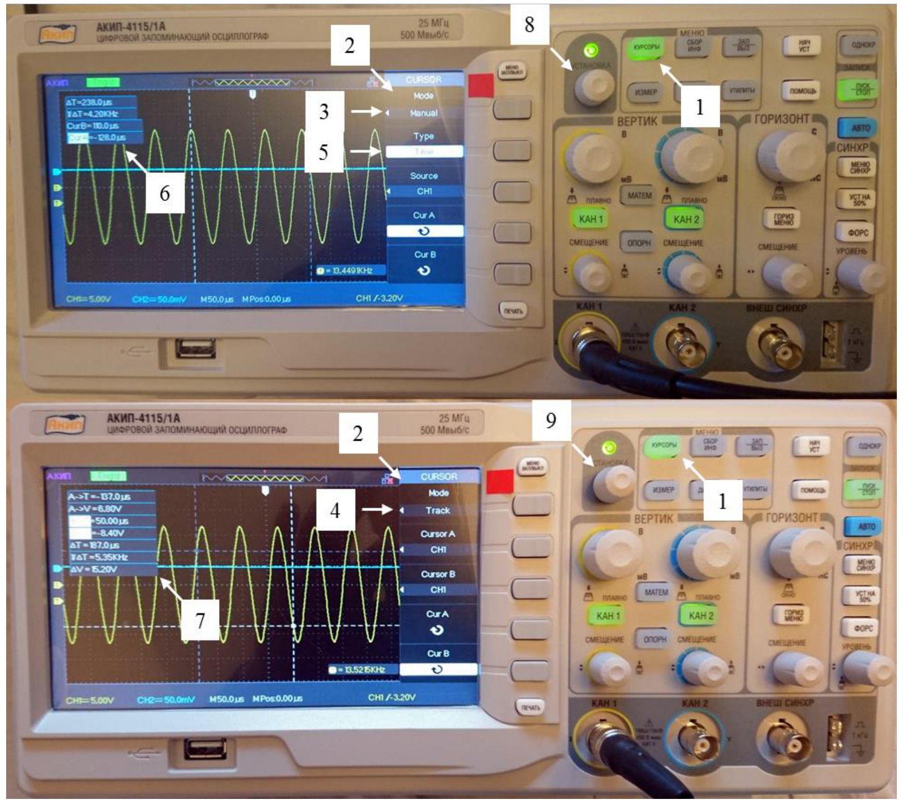
To carry out measurements you may need a cursors menu denoted by «КУРСОРЫ» 2 on Ошибка! Источник ссылки не найден... You may choose yourself either «Manual» 3 on Fig.2) or «Track» (4 on Fig.2) regimes in the menu «Mode» (2 on Fig.2).The second menu in the regime «Manual» allows to regulate the cursor’s axes (5 on Fig.2) In the «Voltage» regime the cursors will move along the vertical axes and will display the values of voltages on the corresponding level. In the regime “Time” the cursors will perform similar functions moving along the horizontal axes. In the regime “Track” the cursors will move along the channel chosen in the second or third items of the menu and will display values of the time and the signal level of the corresponding point. The regulation of the positions of the cursors is realized by turning button «УСТАНОВКА». To switch between the cursors use the two lower grey buttons situated near
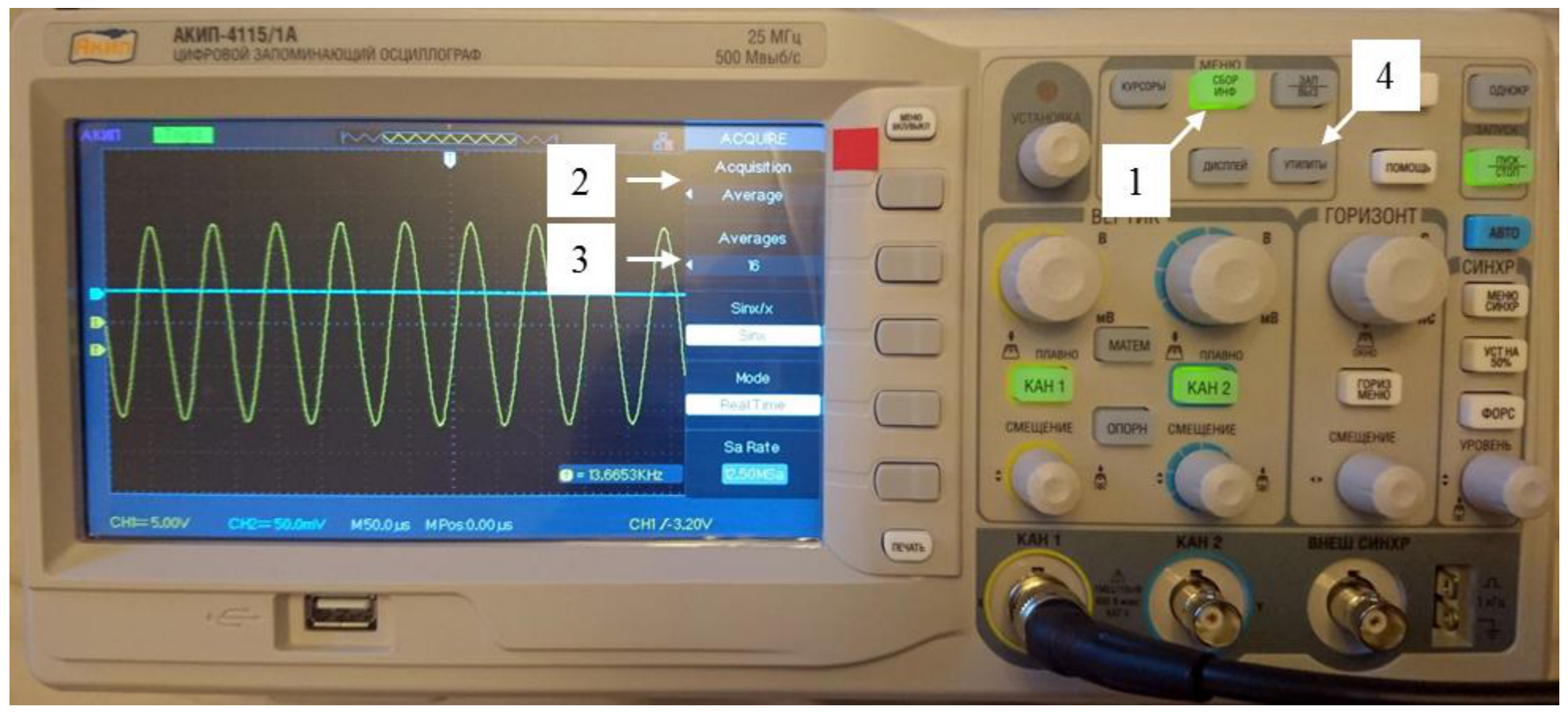
In case your signal is polluted by noise and when its mean position is unstable, you can use the menu collection of information denoted by the knob «СБОР ИНФ» (1 on FigОшибка! Источник ссылки не найден.) and choose the first menu «Acquisition» the regime «Averege» (2 on Ошибка! Источник ссылки не найден.). In that case the signal on the screen will be the average of several sets of signals. The averaged number signals can be chosen in second menu «Avereges» (3 on Fig.3).
Generator
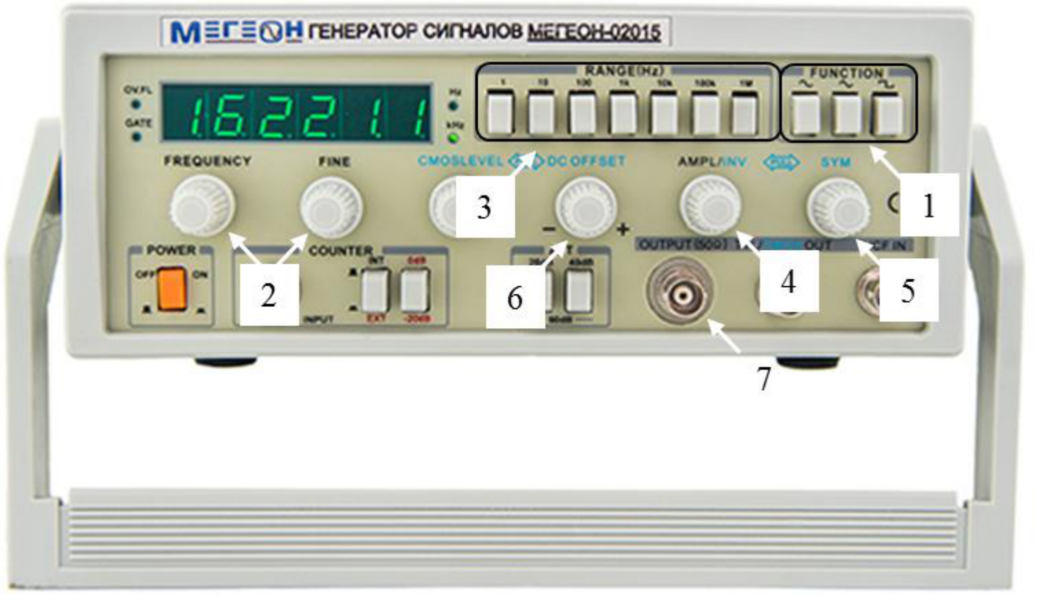
Generator supplies an alternating current of various waveform and frequency to input terminals of electric circuit. Signal type is set by the buttons of sinusoidal, square, and sawtooth signal (1 on Fig.3). Signal frequency is adjusted by buttons «FREQUENCY» and «FINE» (2 on Fig.3). A frequency range is set within the menu «RANGE» (3 on Fig. 3). Button «AMPL/INV» (4 on Fig.3) is used to adjust the signal amplitude. Button «SYM» (5 on Fig.3) in the pull over position allows one to adjust signal symmetry with respect to the point of maximum amplitude (it is recommended to obtain the most symmetric output signal possible). Button «DC OFFSET» (6 on Fig.3) in the pull over position is used to adjust average displacement of the signal voltage with respect to zero (using the button one must set the average voltage to zero). To extract the generator signal to the external circuit, use the socket «OUTPUT ».
Ultrasound receiver/transducer
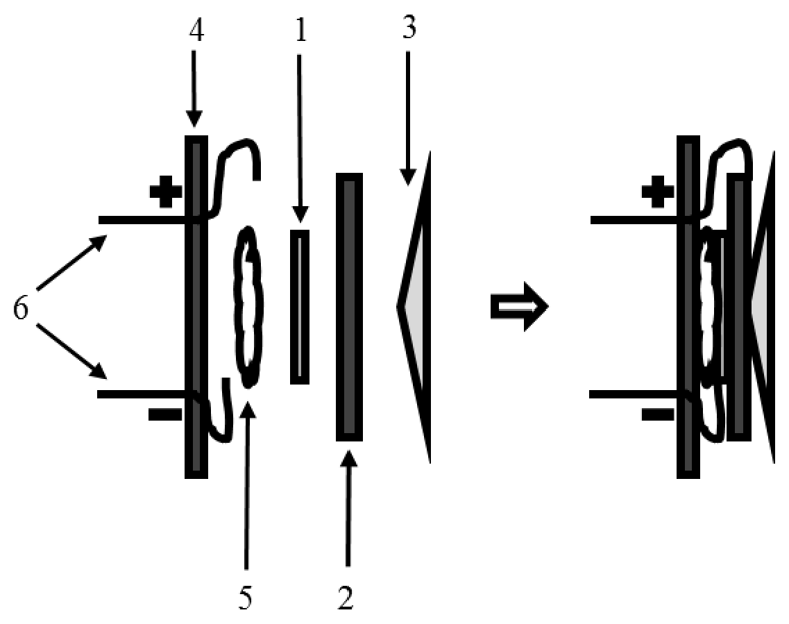
The ultrasonic receiver and transmitter are completely identical, i.e. both can be used as receiver and/or transmitter as well. A detector (see Fig.2) consists of a piezoelectric plate (1), a metal plate (2), a resonator (3) glued to the metal plate, and a base (4) to which the detector is attached by means of an elastic glue (5). The detector terminals (6) are attached to both sides of the piezoelectric plate: directly from one side and through the metal plate to the other side. The detector is rather fragile, the most vulnerable is the contact between the resonator and the metal plate. Please be careful and do not tear the resonator away from the plate during experiment.
Amplifier
It amplifies the magnitude and power of a signal by drawing power from the DC supply unit.
Luxmeter (light intensity) meter
This instrument is designed to measure indoor luminosity. In the experiment it is used as a linear photodetector, i.e. that the light meter readings are proportional to the integrated power of light incident on the probe head. There is a nob “HOLD” on the head of the luxmeter which fixes the reading while that button is in the lower position. To continue the measurements you have to press that button once again to move it to higher position.
Source note: The original manual prints repeated figure numbers and the Russian broken-reference messages “Ошибка! Источник ссылки не найден.” with varying punctuation. Its cursor paragraph stops after “near”. These source defects remain literal; no missing target or sentence ending is supplied.
Equipment list
- An oscilloscope.
- A generator.
- An amplifier.
- Connection wires.
- Coaxial cables of oscilloscope. «Plus» of oscilloscope cable corresponds to the retractable contact and «Minus» to the crocodile clip.
- A coaxial cable of generator.
- An ultrasound receiver and a transducer.
- A rail for detector mounting.
- A wooden sample on the support.
- Pieces of wooden ruler.
- A stand.
- A flashlight.
- Two linear polarisers.
- A circular polariser.
- Turntables for the polarisers.
- A light meter.
- Lasers: violet (wavelength of 405 nm), green (532 nm), and red (650 nm).
- A power supply unit of the lasers and the amplifier.
- Fixing gum
Preface
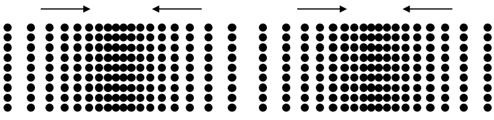
Anisotropy is the dependence of a substance property on direction inside the substance. In this experiment you will study anisotropy of elastic and electrical properties of various substances by means of sound and electromagnetic waves. A sound wave is elastic mechanical wave propagating in a substance. Speed of propagation of sound wave is determined by elastic properties of the substance (i.e. how it responds to mechanical deformation) and its density. If the substance elastic properties are anisotropic, the speed of sound depends on the direction of wave vector. In this experiment only longitudinal sound waves are studied.
Part 1. Sound waves. Measurement of speed of sound by phase method.
Item 1-0 (not evaluated) If you are not familiar with oscilloscope and generator, try to connect the generator and oscilloscope directly. Obtain a stable shape on the display in «Auto» mode for various types of signal from the generator. Try the same using «Single» mode as well.
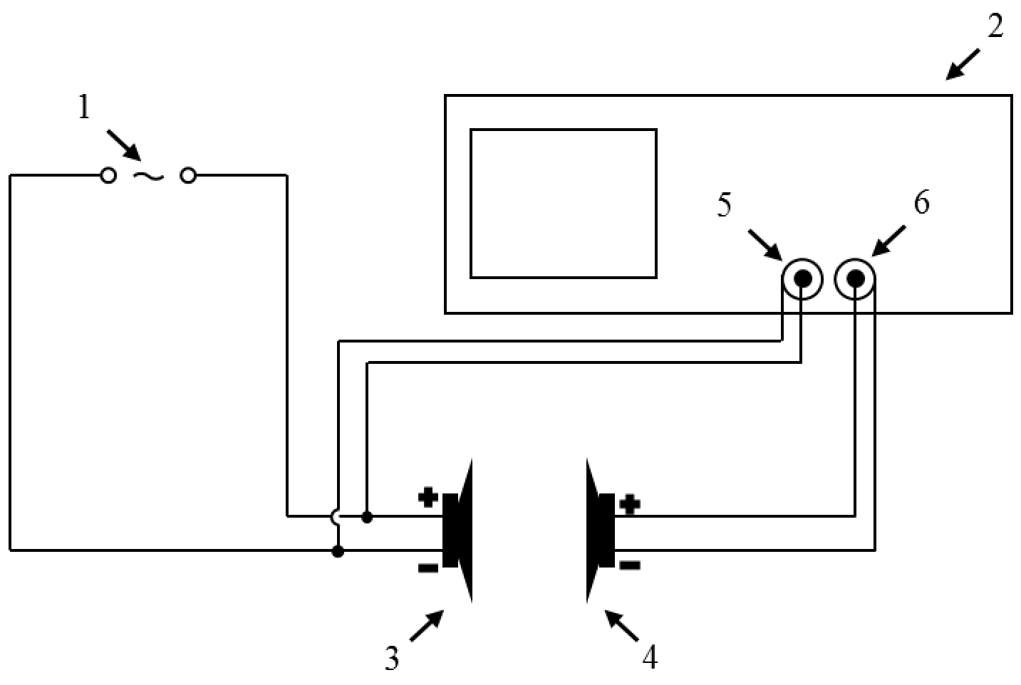
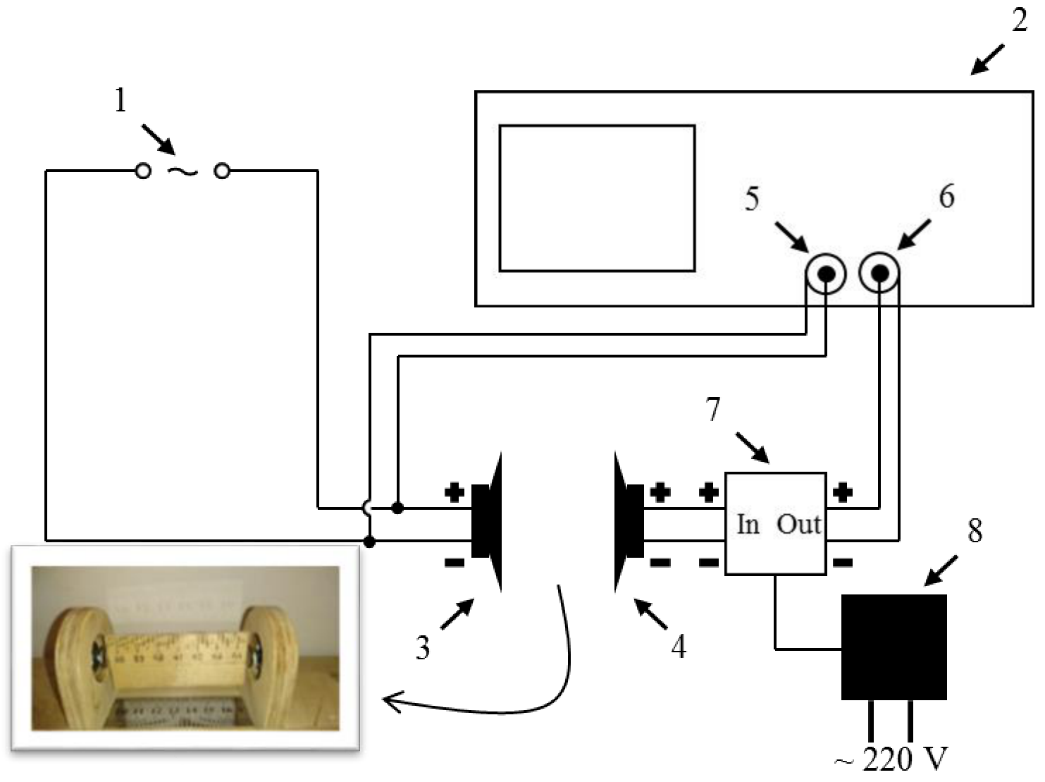
Item 1-1 Mount the receiver and transducer on the rail so that their resonators are facing each other at a distance about 10 cm. Connect the devices according to the circuit diagram shown in Fig.3. Adjust the generator to produce a sinusoidal signal of maximum amplitude. Obtain a stable shape on the oscilloscope display in «Auto» mode at the first channel (the channel connected to the transducer). By varying generator frequency observe the ensuing change of the signal amplitude at the receiver. Determine the generator frequency corresponding to the maximum signal up to three decimal points.
Item 1-2 Try to move the receiver along the rail by holding the generator frequency constant at the value found in 1-1. A signal shape at the receiver channel will move relative to the shape of the transducer signal. By measuring their mutual displacement determine the wavelength of sound wave produced in air by the transducer. At least 5 experimental points must be recorded.
Item 1-3 Write down the equation relating frequency and wavelength of a sinusoidal signal. Evaluate the speed of sound in air using the measurement results.
Item 1-4 (not evaluated) Switch to the «Display» mode. On the second page of settings in the «Format» menu choose XY mode. In this mode the horizontal coordinate of a sample point is proportional to the signal at the first channel and the vertical coordinate to the signal at the second channel. Adjust the scale to obtain equal amplitudes in vertical and horizontal directions.
Item 1-5 Distance variation between the receiver and transducer results in different types of oscilloscope shapes called Lissajous figures. Sketch five different figure types displayed by oscilloscope and determine a corresponding phase shift between transducer and receiver signals.
Part 2. Measurement of speed of sound by pulse method. Anisotropy of speed of sound in wood.
Item 2-1 Switch the generator into the square signal mode. Set a frequency of 2.5 Hz and the maximum amplitude of the signal. Mount the receiver and transducer about 5 cm apart. A small signal from the receiver appears slightly delayed after the vertical slope of the transducer signal (the rising slope of signal shape). Sketch the typical shape of received signal by setting the scale so that the delay between the front slopes of the receiver and transducer signals is about 1/3 of the display width. Indicate the vertical front slope of the transducer signal. Now increase the separation between the receiver and transducer to 10 cm. Sketch the new signal shape in the neighbour window of answer sheet at the same scale. Emphasise the main changes between the second shape and the first one.
Item 2-2 Let us refer to an interval between the vertical front slope of transducer signal and the first peak of receiver signal as time delay. Measure the dependence of time delay on a distance between the transducer and receiver by working in «CURSORS» mode of oscilloscope. Measure the time delay at least for 7 various distances between the transducer and receiver. Plot the obtained dependence and determine graphically the speed of sound in the room air. Determine the proper time delay between the transducer and receiver signals (i.e. at zero separation between the transducer and receiver resonators).
Item 2-3 Insert a piece of wooden ruler between the transducer and receiver (make sure it is being firmly hold in place). Be careful with the resonators since they are easily deformable under pressure and may break away from the metal plates, which would spoil your results. Report to lab supervisor if a resonator has been damaged. Connect the receiver to the amplifier input and do not forget to connect the amplifier to power supply. Connect the second oscilloscope channel to the amplifier output (see Fig.4). Check polarity and the amplifier «In» and «Out» terminals. Verify that after the amplifier has been connected the amplitude of receiver signal increased. By inserting various pieces of wooden ruler measure the time delay versus the length of a ruler piece. Plot the dependence obtained. Determine graphically the speed of sound propagating in wooden ruler and the proper time delay between transducer and receiver signals.
Item 2-4 Measure and write down the diameter of a wooden sample. Mount the sample on the support between the transducer and receiver. Carefully press the transducer and receiver to the sample at opposite points against angular marks . Measure the dependence of time delay between the front slope of transducer signal and the first peak of receiver signal on the rotation angle of the sample. Do the measurements with a step of from to . Write down the formula for the speed of sound in the sample assuming the proper time delay to be the same as that one measured in item 2-3. Evaluate the speed of sound for different directions. Plot a speed of sound versus rotation angle. Determine the minimum and maximum speed. Which directions do these speeds correspond to: «along wood fibers» or «across the fibers»?
Part 3. Electromagnetic waves. Study of unpolarised and linearly polarised light.
Electromagnetic wave is electromagnetic oscillation propagating in space, i.e. oscillating vectors of electric () and magnetic fields (). Electromagnetic wave is transversal for both vectors, in other words vectors and oscillate perpendicularly to the direction of wave propagation and they are orthogonal as well (see Fig.5). For convenience only vector is usually considered.
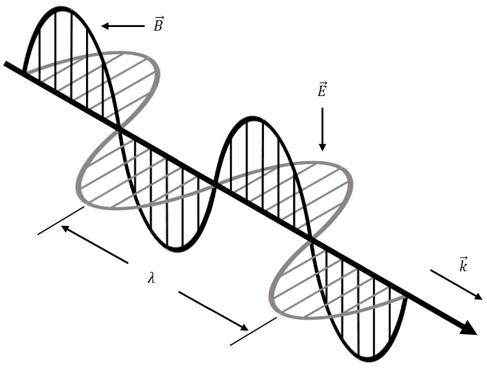
In general light is a superposition of various electromagnetic waves, so the value of electric field vector measured at any moment at some point in space is determined by the principle of superposition. Therefore due to a large number of interfering electromagnetic waves the field intensity varies chaotically. Such a light is called unpolarised. If a wave propagates in a certain direction and its vector oscillates along a certain direction as well, the light is called linearly polarised. The plane defined by the direction of wave propagation and the direction of oscillation of vector is called polarisation plane. Linearly polarised light can be obtained from unpolarised light by transmitting the latter through a linear polariser (LP). This optical device transmits only the component of light wave polarised in a certain plane (i.e. LP is made of a material which is anisotropic with respect to oscillation of electric field vector). The plane is called the transmission plane of LP. The orthogonal component of incident light is absorbed by the polariser. The diagram in Fig.6 illustrates operation principle of LP (the wave propagates from left to right).
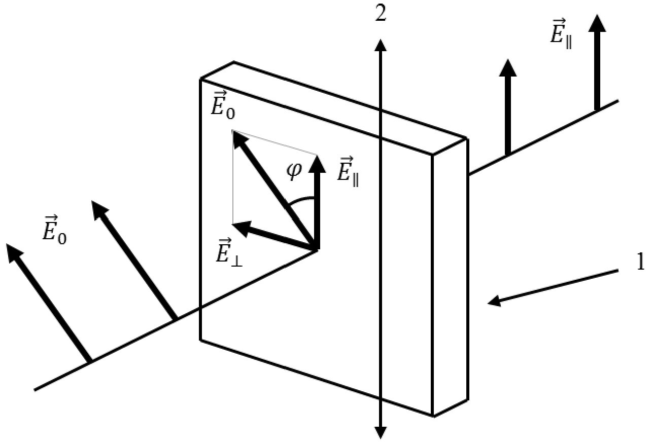
Here is electric field of a linearly polarised incident wave, is the electric field transmitted by the LP, , and is the angle between and .
According to theory of electromagnetic waves light intensity is proportional to the time average of electric field amplitude squared. Therefore intensity of light transmitted by the LP in Fig.6 is determined by intensity of incident light and the angle (Malus’ law):
Item 3-1 Assuming a flashlight to be a source of unpolarised light you should be able to design (make a sketch) and assemble a setup to verify Malus’ law. You have two LPs, a flashlight, a stand, and a light meter. Measure the intensity of light transmitted by the optical setup as a function of the angle between polarisation planes of LPs from to (there must be at least 10 experimental points). Linearise the obtained dependence and plot the points. Verify Malus’ law. The transmission plane of LPs provided is along the line – (see the marks on the LP casing).
Laser light is partially polarised since it contains both linearly polarised and unpolarised components. To describe partially polarised light one can use the concept of degree of polarisation:
where and are maximum an minimum intensities of light transmitted by LP.
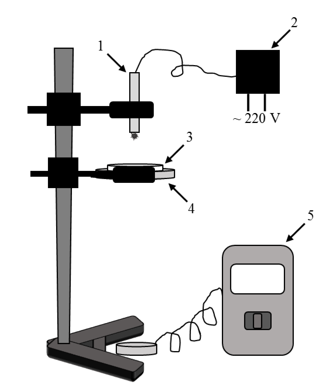
Item 3-2 Assemble the setup for measuring the degree of polarisation of light shown in Fig.7. Measure the degree of polarisation of radiation emitted by the red laser and argue whether the radiation can be regarded as linearly polarised. (Attention! To make sure the intensity of laser radiation has been stabilised and the laser is normally operating wait after the laser was switched on).
Part 4. Study of elliptically polarised light.
Besides linear polarisers there are also circular polarisers (CP). A CP consists of a linear polariser covered with a layer of anisotropic substance (for brevity we refer to this layer as «crystal»). Incident light passes through the LP and the linearly polarised light then passes through the crystal. A light wave in the crystal splits into two (ordinary and extraordinary rays) with orthogonal polarisation planes. The linear polariser and the crystal are so aligned that the intensities (and therefore the electric fields) of ordinary and extraordinary rays are equal. That is transmission plane of the LP included in the CP is at the angle of to polarisation planes of ordinary and extraordinary rays. The crystal is anisotropic: ordinary and extraordinary rays propagate at different speeds. Initially phases of both waves are equal and subsequently a phase shift builds up because of different velocities.
Let and be electric fields of ordinary and extraordinary waves. Using the diagram in Fig.8 consider how superposition of the fields depends on a phase shift between the waves passed through the crystal:
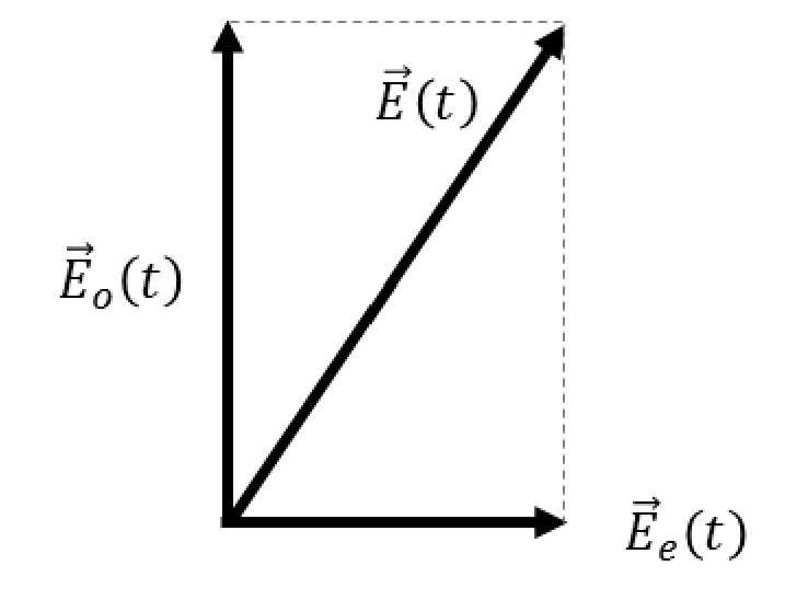
Here and are intensities of electric fields of ordinary and extraordinary waves, is a phase of ordinary wave, is angular frequency of light oscillations, and is the phase shift between the waves.
Item 4-1 Oscillation frequency of vectors and is the same. Which trajectory does the vector follow? Draw all possibilities. What phase shift between ordinary and extraordinary waves correspond to each trajectory?
Light passed through a CP is referred to as elliptically polarised.
Item 4-2 Determine the side of the provided CP on which LP is located. Determine the direction of the LP polarisation plane. Sketch the necessary experimental setup and write a brief explanation (English is preferred but you may use your native language as well). Determine orientation of the transmission plane of the LP according to angular marks on the CP casing.
Item 4-3 Assemble the setup shown in Fig.9 (the LP-side of CP must face the laser!). Rotate the CP until the light transmitted by the CP had maximum intensity. Remember to wait several minutes after the laser power is to stabilise laser output intensity. For all three lasers measure intensity of light transmitted by the system versus the angle between TPs of the LP and the LP built into the CP. Change only LP orientation (for the green laser do the measurement only for maximum and minimum intensities). Plot the dependencies obtained for red and violet lasers on the provided polar coordinate paper for a normalised intensity and indicate laser colour at each plot. Using the dependencies measured determine as best as you can the maximum and minimum light intensity for all three lasers.
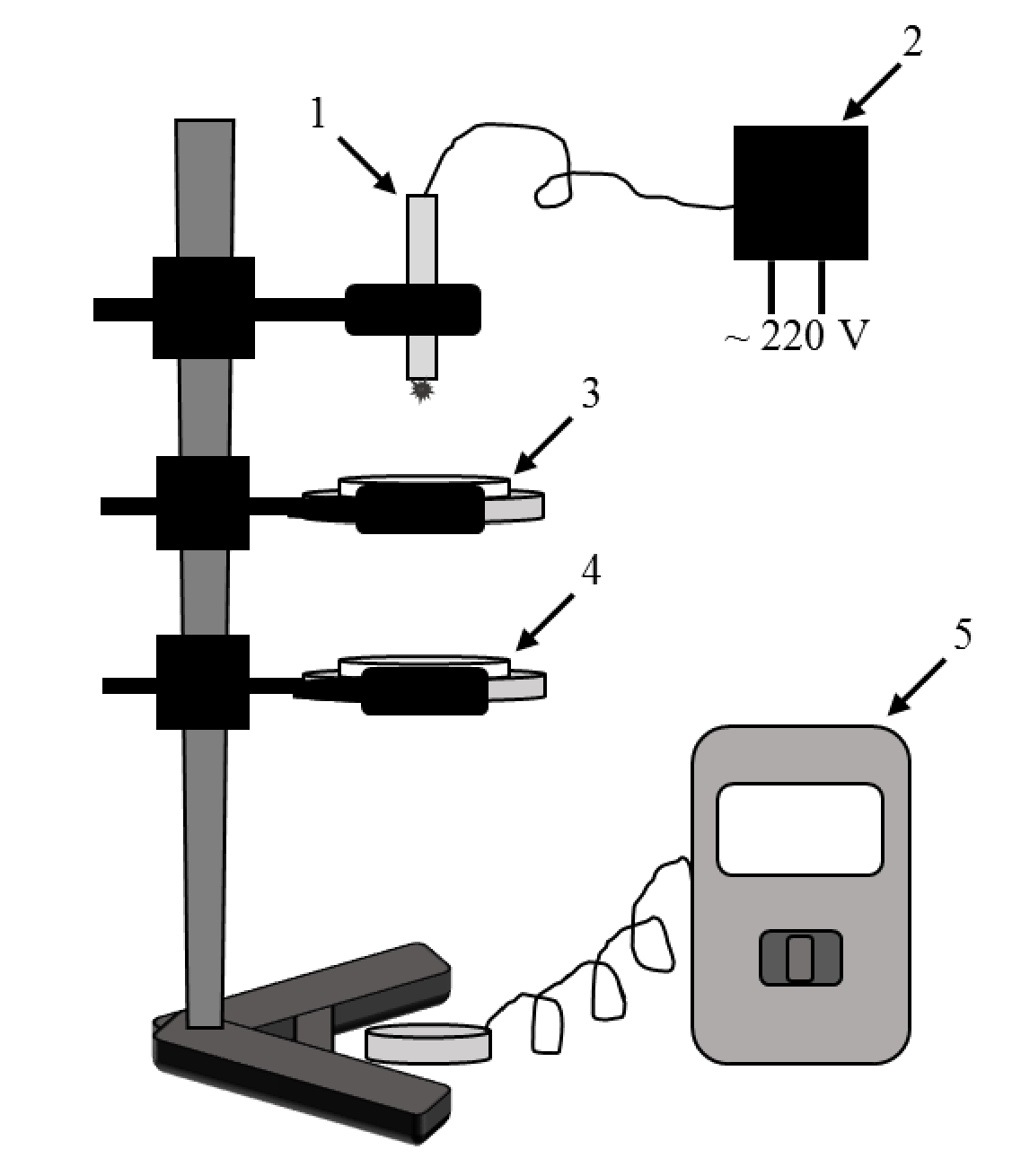
Item 4-4 Derive ordinary and extraordinary waves’ intensity values after passing through LP located after CP. Derive the equation which describes dependencies measured in item 4-3 using the equation which describes interference of two linearly polarised waves of equal frequencies.
where – intensities of two waves polarised in the same plane, - phase shift between these waves.
Item 4-5 Using the maximum and minimum intensities (measured in item 4-3) derive the equation which describes the ratio of elliptical trajectories’ semiaxises for all three lasers and calculate numerical values, plot the analytical dependencies schematically in polar coordinates for all three lasers observing the semiaxes’ lengths ratio and their orientation. is the maximal modulus of . Indicate a plot by the laser colour.
If trajectory of of a wave transmitted by CP is a circle, the wave is called circular polarised and the CP is indeed circular for this particular wavelength.
Let be a phase shift between ordinary and extraordinary waves which passed a CP. Let us express via time intervals it takes a wave to cross the anisotropic crystal:
Here is an angular frequency of the vectors and , and and are time intervals it takes ordinary and extraordinary waves to pass through the crystal, is a wavelength in vacuum (air).
Item 4-6 Write down the equation for the phase shift between ordinary and extraordinary waves acquired on the way through the CP. The equation must include the already measured quantities. Laser wavelengths are written on the equipment list. Evaluate for every wavelength using the data obtained in item 4-3. Plot a linearised dependence of the phase shift on a wavelength and find out for which the CP is indeed the circular polariser.
Решение
Внимание: Непълно решение
The retained key covers all16 evaluated items with full native data/plots/grading, but Point4-5 does not separately print numerical semiaxis ratios requested by Item4-5; original ellipse plots and ratio formula are fully retained. No key for the explicitly unevaluated setup exercises1-0 and1-4 is expected.
The following is the complete matching retained archive key, including its measurement data, original plots/photos and literal marking criteria. No separate organizer URL is retained in this source manifest; the key is attributed to the archive.
Source note: Point 1-3 prints despite giving a sound velocity below. The Point 2-2 graph slope and printed sound velocity differ. Point 2-3 table/plot values and proper delay are retained without refitting. Point 2-4 grades both extreme-velocity ranges under the printed label and gives a minimum of1200m/s alongside a table minimum of1389m/s. Point 3-2 prints94,4±0,6 without a percent sign. Point 4-1 repeats a0,5(*5) grading term despite Total2,5. Point 4-4 changes its intensity prefactor from to literally. Point 4-6 prints “formula in point4-3”, the inconsistent domain , and wavelength-unit headings inµm with405/532/650 numerical entries. The source units/signs/formulas/rubric typos, original plots and data are all preserved below.
Part 1
Point 1-1 Frequency:
Total: 2,5
- 0,5 – dimensions
- 0,5 – correct number of significant figures
- 1,5 – result
- , if
Point 1-2 Measurements and processing:
| , mm | , µs |
|---|---|
| 5 | 0 |
| 10 | 18,10 |
| 15 | 32,26 |
| 20 | 42,50 |
| 25 | 56,70 |
Gradient of the line , whence .
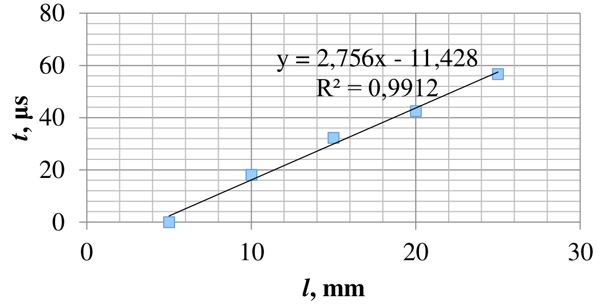
Wavelength: .
Total: 7,0
Measurements: 2,5 – 5 and more points.
If the graph is used:
- 0,5 – scale
- 0,5 – labeled axis
- 1,5 – points are plotted
- 0,5 – error bars
Otherwise 5,5 marks for a method using 5+ points.
- 1,0 – the correct formula for the wavelength
- 0,5 – the answer
Point 1-3 Formula for calculation:
The velocity of the sound in air: .
Total: 3,0
- 1,0 – Formula for calculation
- 0,5 – dimensions
- 1,0 – the answer in the range
- 0,5 for the answer in the range
- 0,5 – the error of the answer is calculated
Point 1-5 The type of the oscillogram / Phase difference:
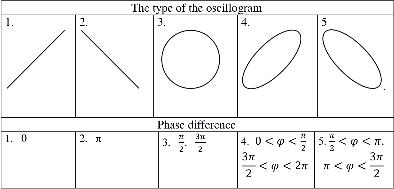
| Phase difference | |
|---|---|
| 1. | |
| 2. | |
| 3. | |
| 4. | , |
| 5. | , |
Total: 5,0
*0,5(5) for each correct diagram.
*0,5(5) for a correct phase difference (even if only one is given).
Part 2
Point 2-1
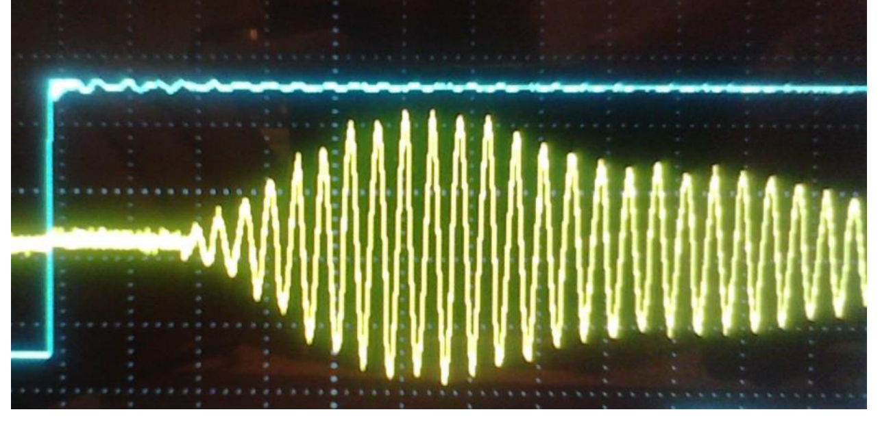
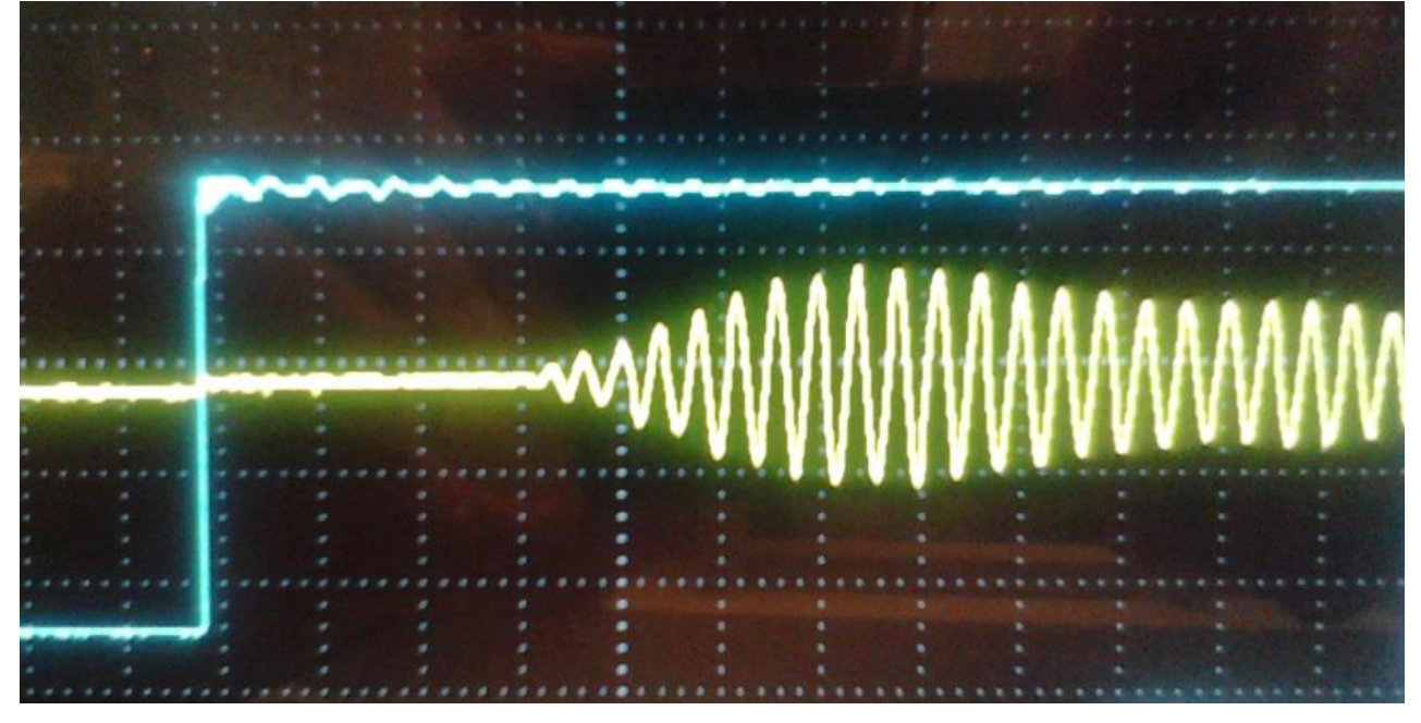
Total: 2,0
- *0,5 (2) for each oscillogram
- 0,5 if can be seen that the delay has grown
- 0,5 if can be seen that the amplitude has decreased
Point 2-2 Measurements:
| , mm | , µs |
|---|---|
| 100 | 358 |
| 90 | 328 |
| 80 | 302 |
| 70 | 272 |
| 60 | 244 |
| 50 | 216 |
| 40 | 188 |
| 30 | 158 |
| 20 | 132 |
| 10 | 106 |
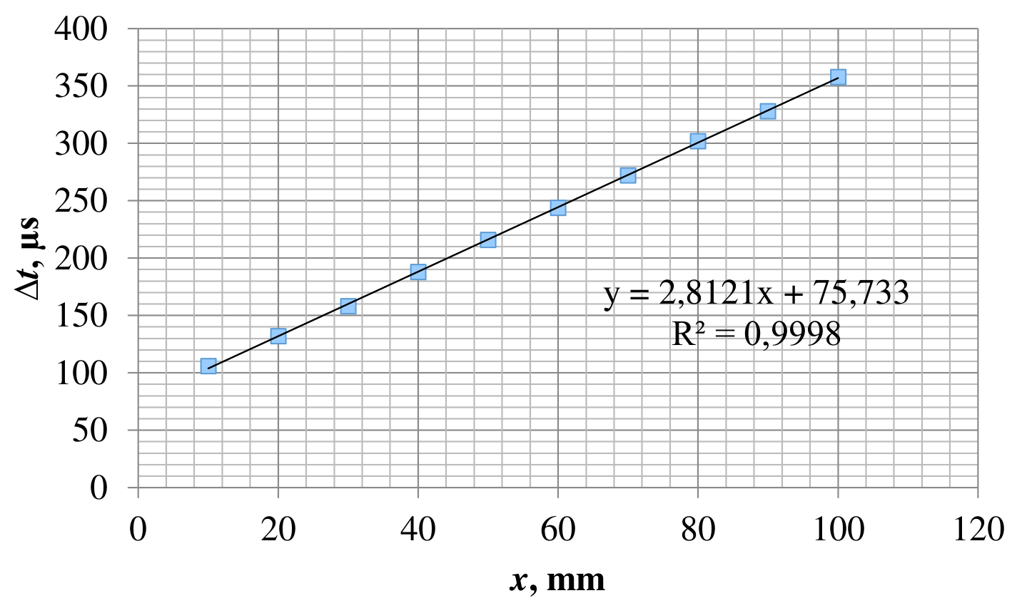
The value of the sound velocity: .
The value of the proper time delay: .
Total: 9,0
- 2,5 – for measurements at 7+ points
- 0,5 – scale
- 0,5 – labeled axis
- 1,5 – points are plotted
- 0,5 – error bars
- 0,5 – dimension of the velocity
- 1,0 – if in the range of
- 0,5 – if in the range of
- 1,0 – determination of the delay time
- 0,5*2 – the error of each answer is calculated ( and )
Point 2-3 Measurements:
| , mm | , µs |
|---|---|
| 236 | 77,2 |
| 130 | 61,8 |
| 113 | 55,4 |
| 70 | 47,6 |
| 40 | 42,2 |
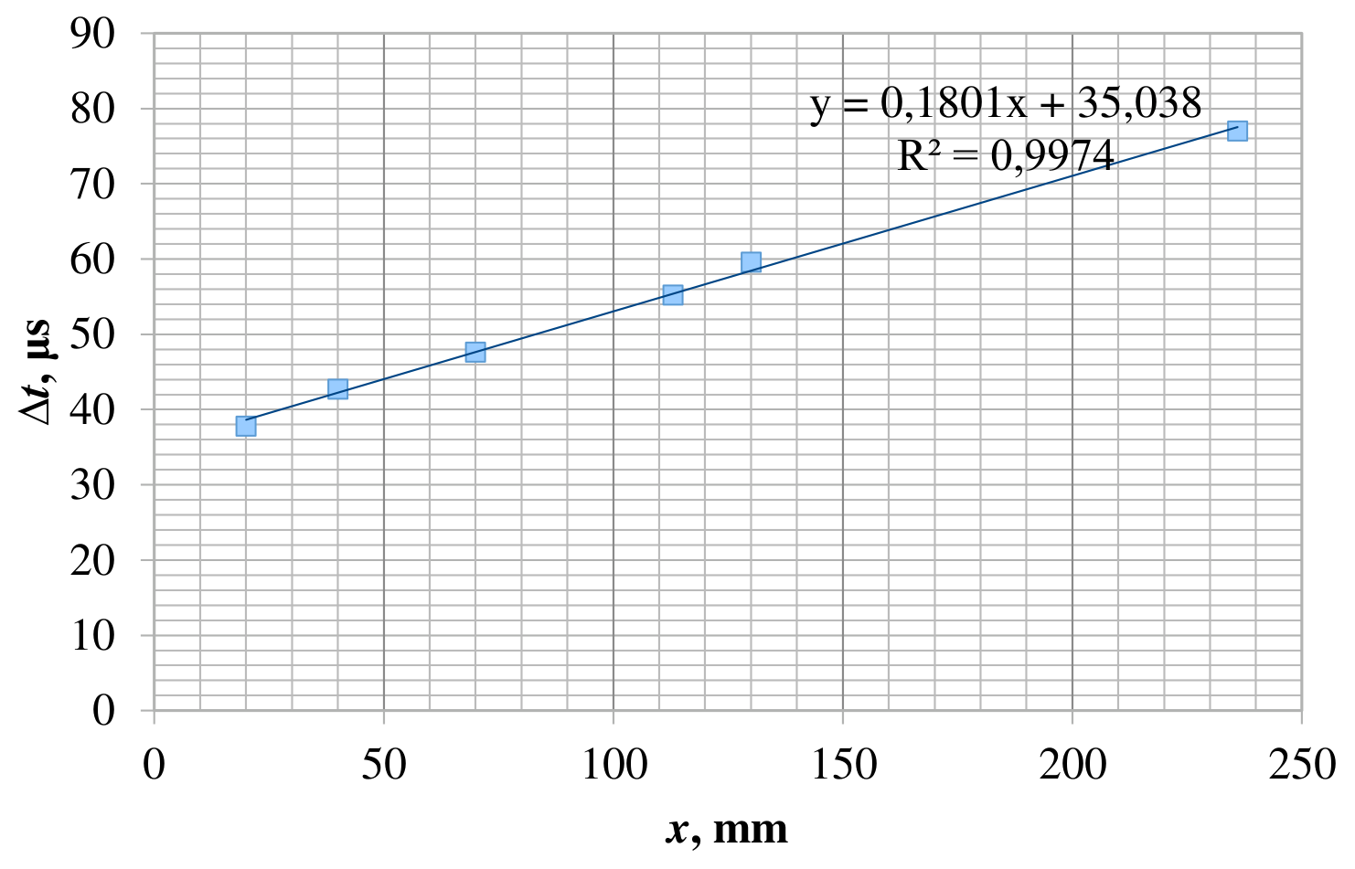
The value of the sound velocity: .
The value of the proper time delay: .
Total: 8,0
- 0,5 for each point (no more than 2,5 marks)
- 0,5 – scale
- 0,5 – labeled axis
- 1,5 – points are plotted
- 0,5 – error bars
- 0,5 – dimensions
- 0,5 – the answer in the range of
- 0,5 – the error of the answer is calculated
- 0,5 – determination of the delay time
- 0,5 – the error of the answer is calculated
Point 2-4 The diameter of the sample: .
Measurements:
| , ° | , µs | , m/s |
|---|---|---|
| 0 | 86,0 | 1961 |
| 15 | 72,0 | 2703 |
| 30 | 103,0 | 1471 |
| 45 | 100,0 | 1538 |
| 60 | 89,5 | 1835 |
| 75 | 71,5 | 2740 |
| 90 | 54,0 | 5263 |
| 105 | 56,5 | 4651 |
| 120 | 92,0 | 1754 |
| 135 | 96,0 | 1639 |
| 150 | 101,0 | 1515 |
| 165 | 107,0 | 1389 |
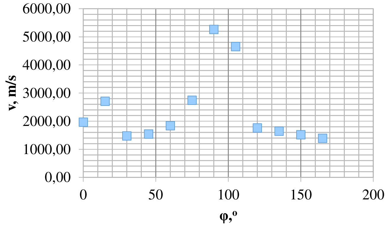
Formula for calculation of the sound velocity:
| Maximum sound velocity | Minimum sound velocity |
|---|---|
| 5300 m/s | 1200 m/s |
| The direction (select the correct answer): • along the wood fibers; across the wood fibers | The direction (select the correct answer): • along the wood fibers; • across the wood fibers |
Total: 13,5
- 0,5 for the diameter in the range of
- 0,5 mark for each point but no more than 5
- 1,0 for correct formula
- 1,0 for using the delay time for rules (0,5 for each of two last points if the delay time wasn’t considered)
- 0,5 – scale
- 0,5 – labeled axis
- 1,5 – points are plotted
- 0,5 – correct characteristic behavior (the presence of a peak at –, allow 1–2 «missing» points)
- 1,0 for in the range of
- 1,0 for in the range of
- 1,0 for correct directions
Source note: The source answer cells print the bullet placement shown above without an explicit selected/crossed answer. No selection is invented.
Part 3
Point 3-1
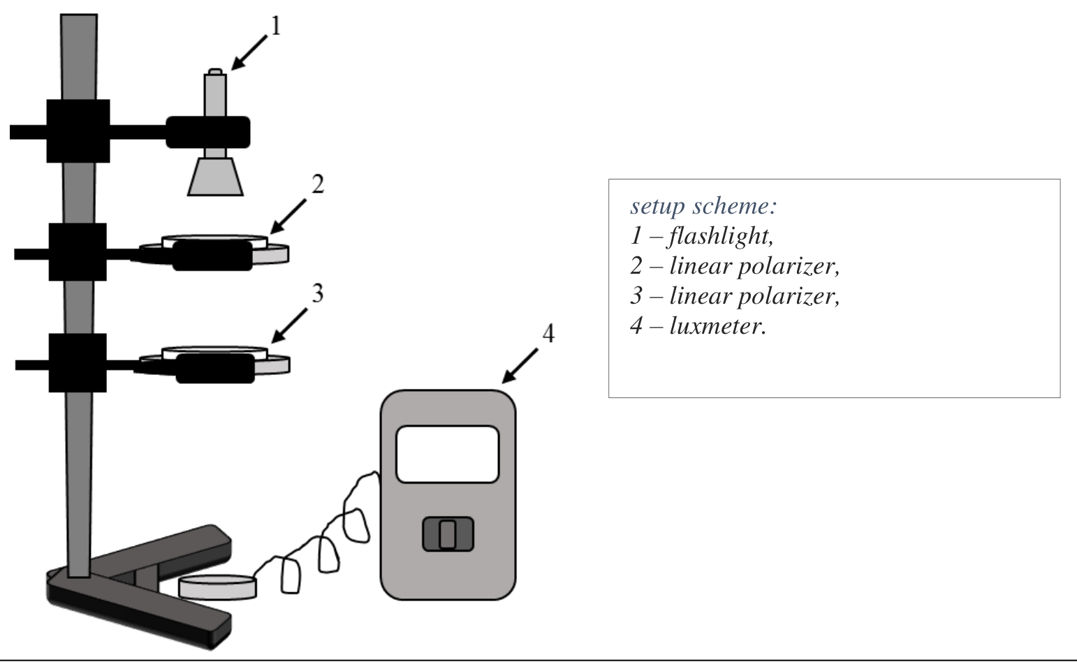
setup scheme: 1 – flashlight, 2 – linear polarizer, 3 – linear polarizer, 4 – luxmeter.
Measurements and processing:
| , ° | , a.u. | |
|---|---|---|
| 0 | 1,00 | 2420 |
| 30 | 0,75 | 1810 |
| 60 | 0,25 | 687 |
| 90 | 0,00 | 129 |
| 110 | 0,12 | 399 |
| 140 | 0,59 | 1390 |
| 170 | 0,97 | 2270 |
| 200 | 0,88 | 2080 |
| 260 | 0,03 | 218 |
| 310 | 0,41 | 980 |
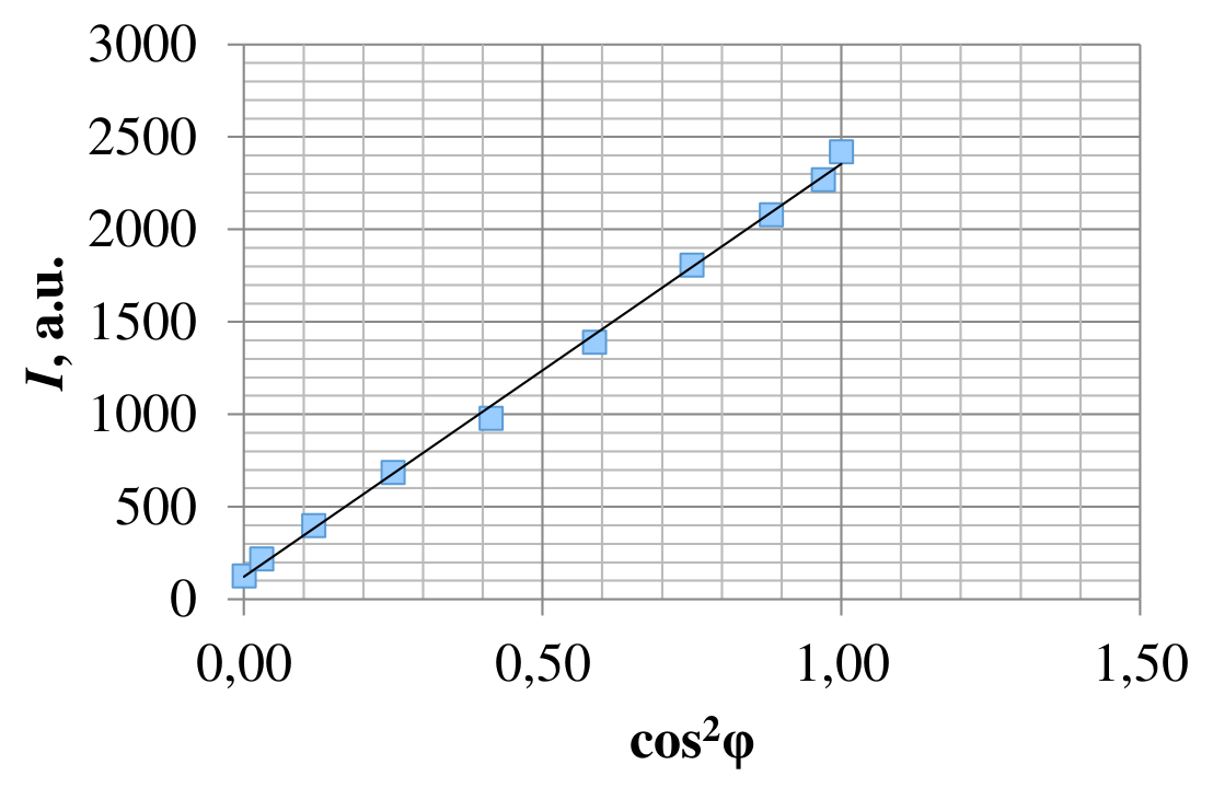
Total: 8,0
- 1,5 for correct experimental setup scheme
- 2,5 for point
- 1,0 – correct linearization
- 0,5 – scale
- 0,5 – labeled axis
- 1,5 – points are plotted
- 0,5 – the graph is linear
Point 3-2
Total: 2,0
- 0,5 for each value of
- 0,5 for determined
- 0,5 – errors
Part 4
Point 4-1 The type of the oscillogram / Phase difference:
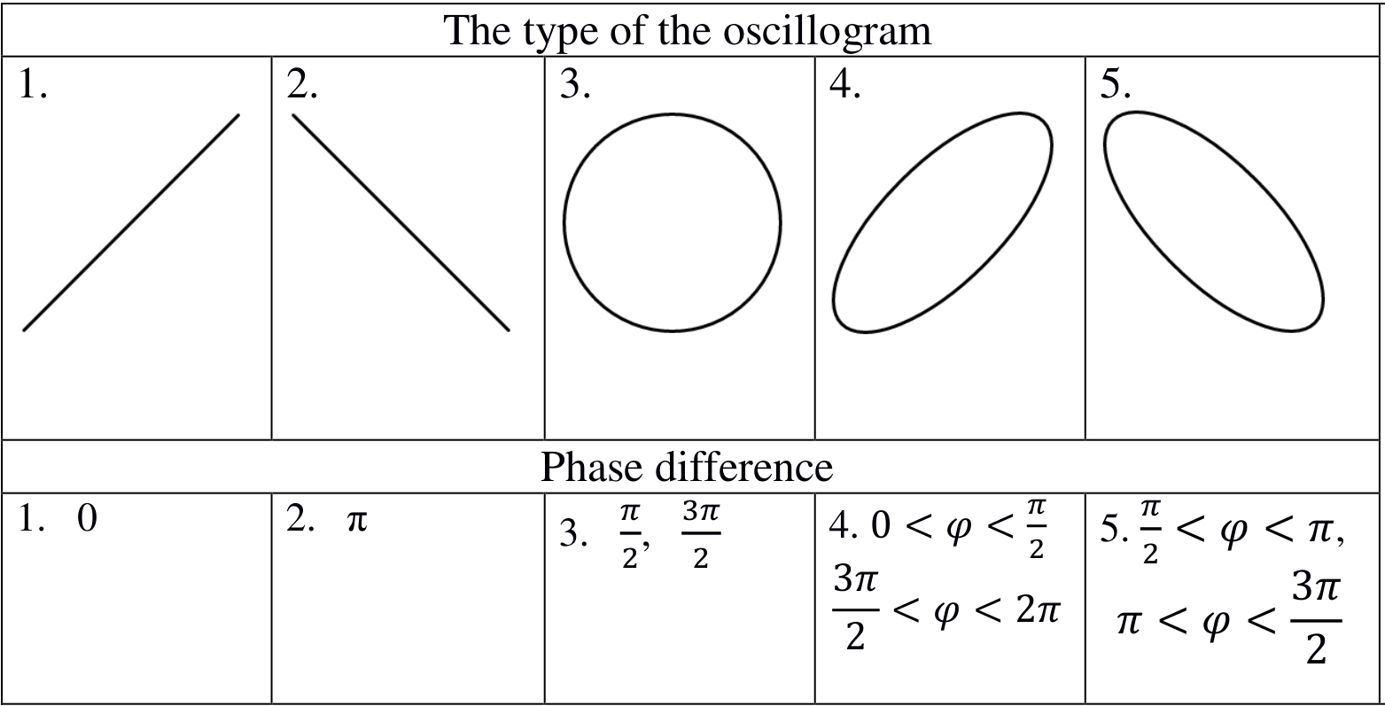
| Phase difference | |
|---|---|
| 1. | |
| 2. | |
| 3. | |
| 4. | , |
| 5. | , |
Total: 2,5
0,5(5) 0,5( 5) for each correct diagram + corresponding correct phase difference (even if only one is given).
Point 4-2 The scheme of the experiment and a short text comment:
Experimental setup:
- laser
- power supply
- circular polarizer
- stand
- luxmeter
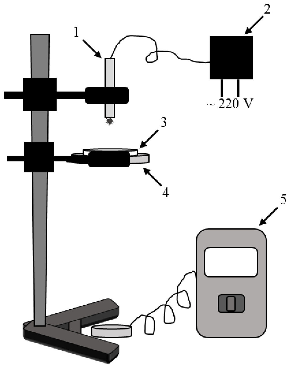
If the Linear polarizer (LP) is closer to the laser, then there exists an angle for which you get very small value of the intensity when the polarization of the laser beam and LP polarization plane (PP) are perpendicular. If the circular polarizer (CP) is closer to the laser, then such an angle doesn’t exist
The position of the polarization plane (PP) of the LP (in degrees on the scale of the CP holder) . (Can be found by crossing LP and LP in CP: ( (crystall–LP)–LP) ).
Total: 5,0
- 3,5 – correct method (if an alternative method is proposed total mark is given)
- 0,5 for determination of the angle
- 1,0 for values in the range
- 0,5 if the answer in the range
Point 4-3 Minimum and maximum intensities (a.u.)
| Red | Green | Violet | |
|---|---|---|---|
| Maximum | 1026 | 56 | 92 |
| Minimum | 410 | 45 | 39 |
Measurements for the red laser:
| , ° | , a.u. | |
|---|---|---|
| 0 | 960 | 0,936 |
| 10 | 909 | 0,886 |
| 20 | 799 | 0,779 |
| 30 | 734 | 0,715 |
| 40 | 616 | 0,600 |
| 50 | 520 | 0,507 |
| 60 | 463 | 0,451 |
| 70 | 425 | 0,414 |
| 80 | 410 | 0,400 |
| 90 | 440 | 0,423 |
| 100 | 476 | 0,464 |
| 110 | 568 | 0,554 |
| 120 | 660 | 0,643 |
| 130 | 741 | 0,722 |
| 140 | 822 | 0,801 |
| 150 | 905 | 0,882 |
| 160 | 969 | 0,944 |
| 170 | 980 | 0,955 |
| 180 | 962 | 0,938 |
Measurements for violet laser:
| , ° | , a.u. | |
|---|---|---|
| 0 | 39 | 0,424 |
| 10 | 43 | 0,467 |
| 20 | 50 | 0,543 |
| 30 | 58 | 0,630 |
| 40 | 67 | 0,728 |
| 50 | 77 | 0,837 |
| 60 | 84 | 0,913 |
| 70 | 90 | 0,978 |
| 80 | 92 | 1,000 |
| 90 | 91 | 0,989 |
| 100 | 87 | 0,946 |
| 110 | 80 | 0,870 |
| 120 | 73 | 0,793 |
| 130 | 63 | 0,685 |
| 140 | 53 | 0,576 |
| 150 | 45 | 0,489 |
| 160 | 41 | 0,446 |
| 170 | 39 | 0,424 |
| 180 | 41 | 0,446 |
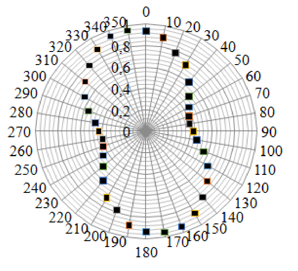
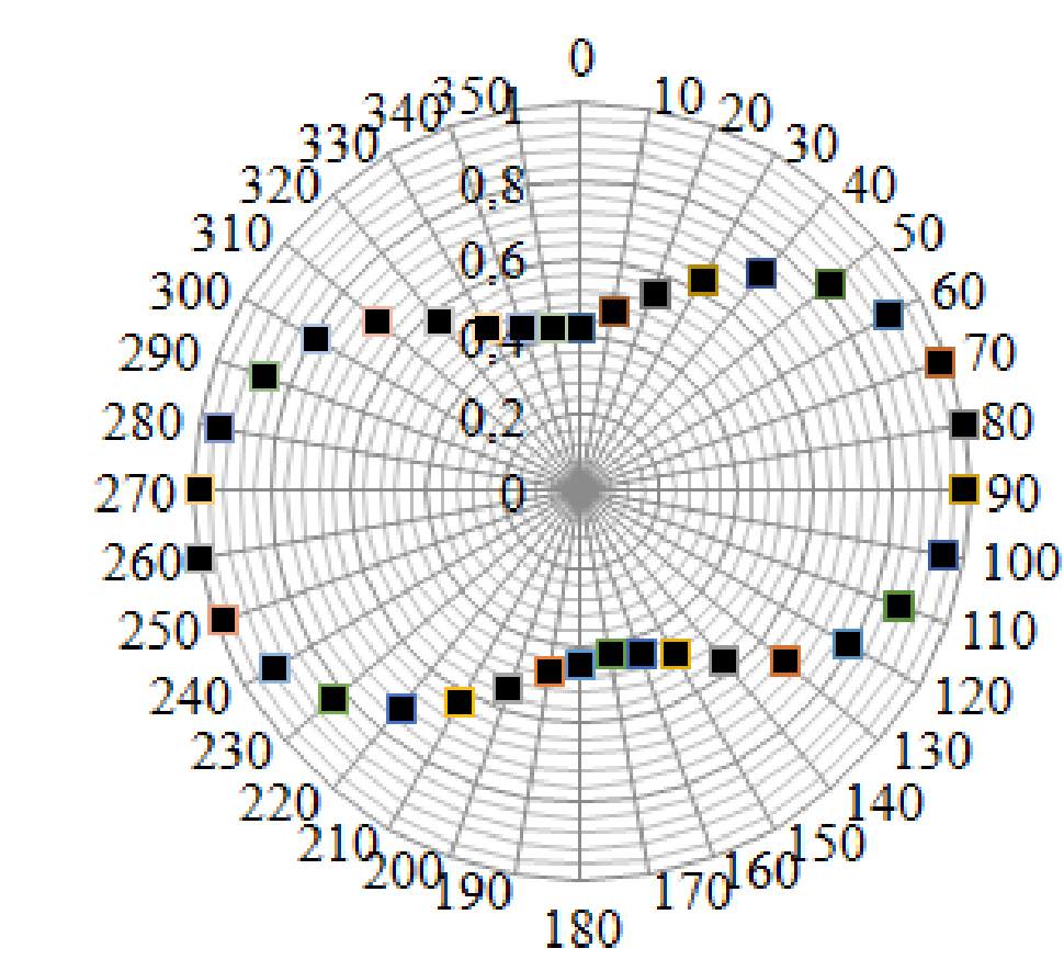
Total: 13,0
(0,52) 3=3,0 For finding maxima and minima.
Dependence for the red laser:
- 2,5 – 20+ points
- 1,5 – 15+ points
- 0,5 – 5+ points
(if measured for n points and is mentioned, the values for the symmetrical points are the same, marks are given for 2n points)
- 1,0 – normalized to
- 1,0 – points are plotted on the graph
- 0,5 – the correct characteristic shape of the graph («bob»)
The dependence for the violet laser is marked similar to the criteria of the red laser
Point 4-4 Derivation of the formula:
Let – be the angle between CP and LP in CP (equal to ). Then if after LP in CP the amplitude of the wave is , then the amplitudes of ordinary and extraordinary waves are equal to and correspondingly
During the passage the amplitudes do not change ( we ignore this effect) and the ordinary and extraordinary waves differ only by a phase shift of .
This waves pass through the LP and we get for the amplitudes of ordinary and extraordinary waves
correspondingly.
. Taking into account the interference of the waves which passed through the polarizer we get (by inserting ):
where .
From the latter we obtain
Total: 5,0
- 1,0*2 for expressions for the intensities and or for corresponding amplitudes
- 3,0 for derivation of the final formula (–1,0 mark for incorrect angle in the formula)
Any alternative derivation giving the correct final formula is given a total mark
Point 4-5 Since the intensity is proportional to the square of the amplitude we have .
From this knowing the ratio of maximum and minimum intensities from Point 4-3 for each of the laser we can obtain the ratio of the ellipse semiaxis. Also from the measurements in point 4-3 know the orientation of the ellipse relative to polarization plane of LP in CP. This allows to sketch the ellipses.
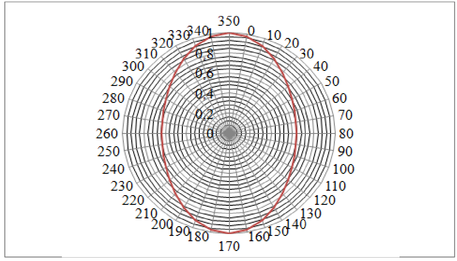
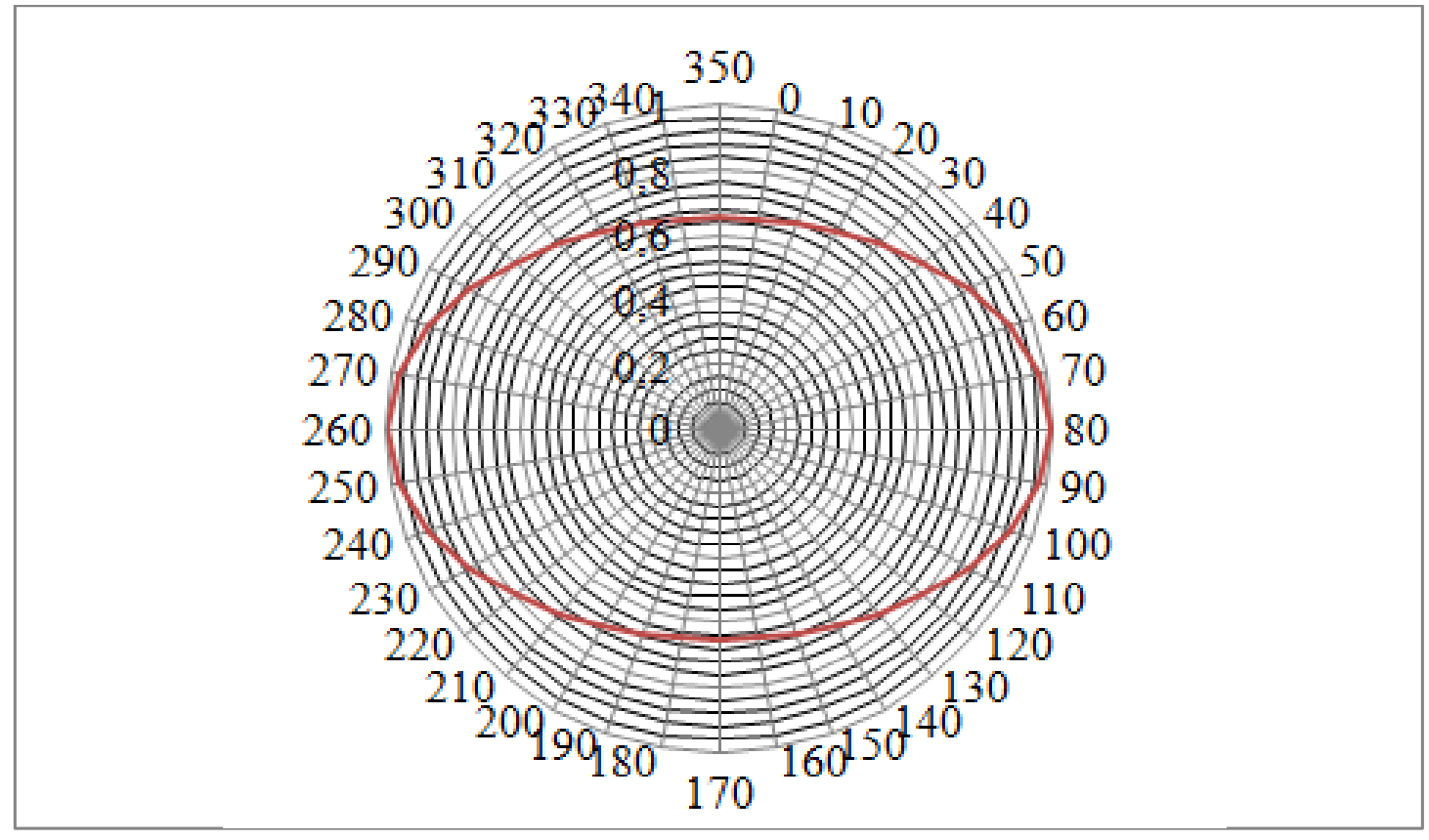
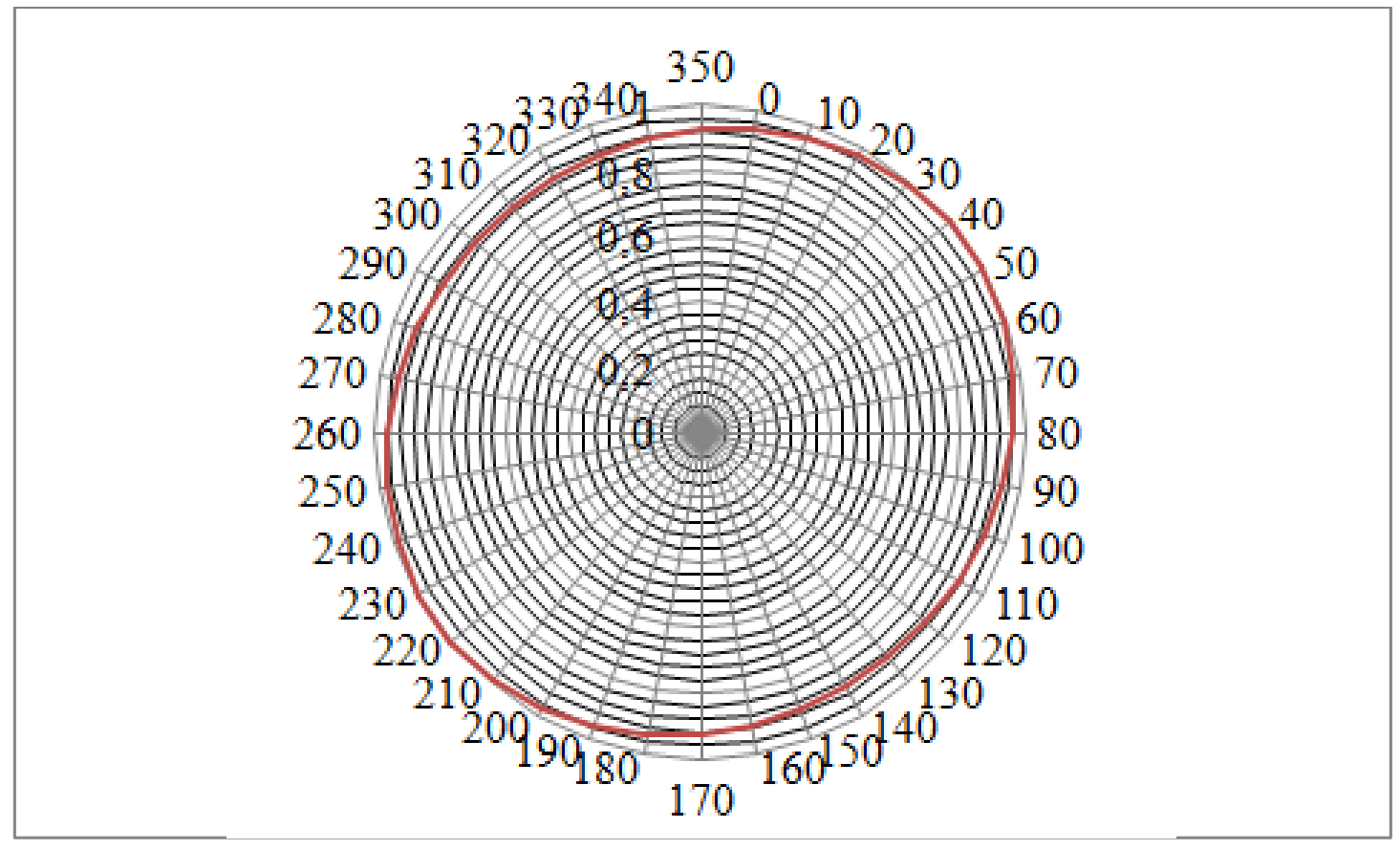
Total: 3,5
0,5 for derivation of the formula.
1*3=3,0 for points plotted on 3 graphs:
- –0,5 for correct orientation of the semiaxis
- –0,5 for correct ratio of the semiaxis
Source note: The retained key provides the three native ellipse plots and the ratio formula; it does not print separate numerical semiaxis ratios requested in Item4-5. No computed additions are attributed to this key.
Point 4-6 Formula:
From formula in point 4-3 it follows, that for
Then
From which we get
At and interchange and the required
(this takes place for violet color).
Draw a graph , taking into account that point for the green color isn’r very reliable because of the instability of the intensity of the laser:
| , µm | , µm⁻¹ | , ° | , ° |
|---|---|---|---|
| 405 | 0,00247 | 113,8 | 1,2 |
| 532 | 0,00188 | 84 | 15 |
| 650 | 0,00154 | 64,6 | 8 |
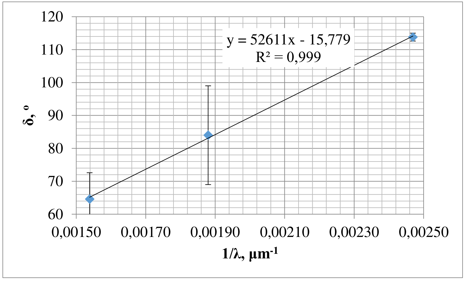
Wavelength:
Getting from the graph the value for the , we obtain the required wavelength:
.
Total: 11
- 2,0 for pointing then maximum and minimum
- 2,0 for any mentioning of using the supplementary angle for violet color
- 1,5 – the table
- 0,5 – scale
- 0,5 – labeled axis
- 1,5 – points are plotted
- 0,5 – error bars
- 2,0 – the answer in the range of
- 1,0 – the answer in the range of
- 0,5 – error is calculated
Total: 100
Оригинал в Архива: prak.pdf · решение от архива: phys-prak-sol-en.pdf