Съдържание

Условие Отговори Решение

IPhO 1986, Експеримент — Задача 2. EXPERIMENT 2

Оригинал на условието (PDF)Съобщи за грешка

Всички материали от IPhO 1986

1986 INTERNATIONAL PHYSICS OLYMPIAD

Условие

Apparatus

RML Nimbus computer

Ten sheets of graph paper.

Please complete synopsis sheet in addition to answering this experimental problem.

THIS IS A TWO AND A HALF HOUR EXAMINATION

INFORMATION

The microcomputer has been programmed to solve the Newtonian equations of motion for a two-dimensional system of 25 interacting particles, in the xy plane. It is able to generate the positions and velocities of all particles at discrete, equally spaced time intervals. By depressing appropriate keys (which will be described), access to dynamic information about the system can be obtained.

The system of particles is confined to a box which is initially (at time $t = 0$ ) arranged in a two-dimensional square lattice. A picture of the system is displayed on the screen together with the numerical data requested. All particles are identical; the colours are to enable the particles to be distinguished. As the system evolves in time the positions and velocities of the particles will change. If a particle is seen to leave the box the program automatically generates a new particle that enters the box at the opposite face with the same velocity, thus conserving the number of particles in the box.

Any two particles i and j, separated by a distance $r_{ij}$ interact with a well-defined potential $U_{ij}$ ,

It is convenient to use dimensionless quantities throughout the computation. The quantities given below are used throughout the calculations.

Variable	Symbol
Distance	$r^*$
Velocity	$v^*$
Time	$t^*$
Energy	$E^*$
Mass of particle	$M^* = 48$
Potential	$U_\mathrm{ij}^*$
Temperature	$T^*$
Kinetic Energy	$E_k^* = \frac{1}{2}m^v^{2}$

INSTRUCTIONS

The computer program allows you to access three distinct sets of numerical information and display them on the screen. Access is controlled by the grey function keys on the left-hand side of the keyboard, labelled F1, F2, F3, F4, and F10. These keys should be pressed and released - do not hold down a key, nor press it repeatedly. The program may take up to 1 second to respond.

FIRST INFORMATION SET. PROBLEMS 1 – 5

\langle v_x, n\rangle = \frac{1}{25}\sum_{i=1}^{25}\left(v_{ix}^*\right)^n

\langle v_y, n\rangle = \frac{1}{25}\sum_{i=1}^{25}\left(v_{iy}^*\right)^n

and

\langle U\rangle = \frac{1}{25}\sum_{j=1}^{25}\ \sum_{i=1}^{25}U_{ij}^* \qquad (i \neq j)

where

$v_{ix}^*$ is the dimensionless x – component of the velocity for the i’th particle,

$v_{iy}^*$ is the dimensionless y – component of the velocity for the i’th particle,

and n is and integer with $n \geq 1$ .

[Note: the summation over $U_{iy}^*$ excludes the cases in which $i = j$ ]

After depressing F1 it is necessary to input the integer $n\ (n \geq 1)$ by depressing one of the white keys in the top row of the keyboard, before the information appears on the screen.

The information is displayed in dimensionless time intervals $\Delta t$ at dimensionless times

$S\,\Delta t^{**}$ (S = 0, 1, 2, .....)

$\Delta t^{**}$ is set by the computer program to the value $\Delta t^{**} = 0{\bullet}100000$ .

The value of S is displayed at the bottom right hand of the screen. Initially it has the value S = 0. The word "waiting" on the screen indicates that the calculation has halted and information concerning the value of S is displayed.

Depressing the long bar (the "space" bar) at the bottom of the keyboard will allow the calculation of the evolution of the system to proceed in time steps $\Delta^{**}t$ . The current value of S is always displayed on the screen. Whilst the calculation is proceeding the word "running" is displayed on the screen.

Depressing F1 again will stop the calculation at the time integer indicated by S on the screen, and display the current values of

\langle v_x,n\rangle,\ \langle v_y,n\rangle \text{ and } \langle U\rangle

after depressing the integer n. The evolution of the system continues on pressing the long bar.

The system can, if required, be reset to its original state at S = 0 by pressing F10 TWICE.

SECOND INFORMATION SET: PROBLEM 6

Depressing F2 initiates the computer program for the compilation of the histogram in problem 6. This program generates a histogram table of the accumulated number $\Delta N$ , of particle velocity components as a function of dimensionless velocity. The dimensionless velocity components, $v_x$ and $v_y$ are referred to collectively by $v_c$ . The dimensionless velocity range is divided into equal intervals $\Delta v_c = 0.05$ . The centres of the dimensionless velocity "bins" have magnitudes

v_c^* = \mathrm{B}\Delta v_c^* \qquad (\mathrm{B} = 0,\pm 1\ \pm 2,..........)

When the long bar on the keyboard is pressed the 2 x 25 dimensionless velocity components are calculated at the current time step, and the program adds one, for each velocity component, into the appropriate velocity 'bin'. This process is continued, for each time step, until F3 is depressed. Once F3 is depressed the (accumulated) histogram is displayed. The accumulation of counts can then be continued by pressing the long bar. (Alternatively if you wish to return to the initial situation, with zero in all bins, press F2).

The accumulation of histogram data should continue for about 200 time steps after initiation.

In the thermodynamic equilibrium the histogram can be approximated by the relation

\Delta N = A e^{\left[\frac{-24(v_c^*)^2}{\alpha}\right]}

where $\alpha$ is a constant associated with the temperature of the system, and A depends on the total number of accumulated velocity components.

THIRD INFORMATION SET: PROBLEM 7

Depressing F4 followed by the long bar at any time during the evolution of the system will initiate the program for Problem 7. The program will take some 30 seconds, in real time, before displaying a table containing the two Quantities

\langle RX,2\rangle = \frac{1}{25}\sum_{i=1}^{25}\left[x_i^*(S) - x_i^*(SR)\right]^2

and

\langle RY,2\rangle = \frac{1}{25}\sum_{i=1}^{25}\left[y_i^*(S) - y_i^*(SR)\right]^2

where $x_\mathrm{i}^*$ and $y_\mathrm{i}^*$ are the dimensionless position components for the i'th particle. S is the integer time unit and SR is the fixed initial integer time at which the programme is initiated by depressing F4. It is convenient to introduce integer

$SZ = S - SR$ ..

The programme displays a table of $\langle RX,2\rangle$ and $\langle RY,2\rangle$ for

$SZ = 0, 2, 4$ ..……24.

Prior to the display appearing on the screen a notice 'Running' will appear on the screen indicating that a computation is proceeding. Depressing F4, followed by the long bar, again will initiate a new table with SR advanced to the point at which F4 was depressed.

COMPUTATIONAL PROBLEMS

1 Verify that the dimensionless total linear momentum of the system is conserved for the times given by

S = 0, 40, 80, 120, 160.

State the accuracy of the computer calculation.

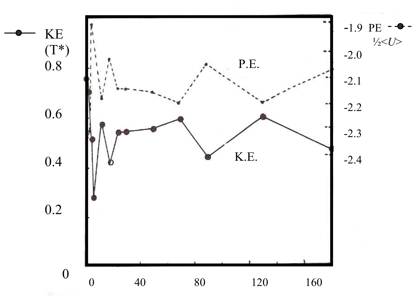
2. Plot the variation in dimensionless kinetic energy of the system with time using the time sequence

S = 0, 2, 4, 6, 12, 18, 24, 30, 50, 70, 90, 130, 180.

3. Plot the variation in dimensionless potential energy of the system with time using the time sequence in 2.

4. Obtain the dimensionless total energy of the system at times indicated in 2. Does the system conserve energy? State the accuracy of the total energy calculation.

5. The system is initially (at $S = 0$ ) NOT in thermodynamic equilibrium. After a period of time the system reaches thermodynamic equilibrium in which the total dimensionless kinetic energy fluctuates about a mean value of $E_k^*$ . Determine this value of $E_k^*$ and indicate the time, SD, after which the system is in thermodynamic equilibrium.

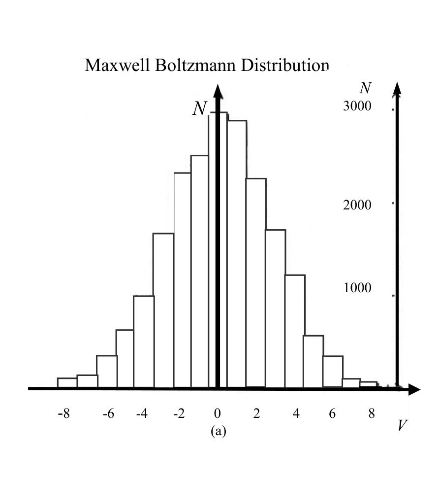
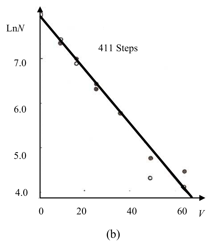
6. Using the dimensionless accumulated velocity data, during thermodynamic equilibrium, draw up a histogram giving the number $\Delta N$ of velocity components against dimensionless velocity component, using the constant velocity component interval $\Delta V_c^* = 0.05$ , specified in the table available from the SECOND INFORMATION SET. Data accumulated from approximately 200 time steps should be used and the starting time integer S should be recorded.

Verify that $\Delta N$ satisfies the relation

\Delta N = A e^{-\left[\frac{24(v_C^*)^2}{\alpha}\right]}

where C and A are constants. Determine the value of $\alpha$ .

7. For the system of particles in thermodynamic equilibrium evaluate the average value of $R^2$ , $\langle R^2\rangle$ , where R is the straight line distance between the position of a particle at a fixed initial time number SR and time number S. The time number difference $SZ = (S - SR)$ takes the values

SZ = O, 2, 4, ….. 24.

Plot $\langle R^2\rangle$ against SZ for any appropriate value of SR. Calculate the gradient of the function in the linear region and specify the time number range for which this gradient is valid.

In order to improve the accuracy of the plot repeat the previous calculations for three (additional) different values of SR and determine the AVERAGE $\langle R^2\rangle$ for the four sets of results together with the 'linear' gradient and time number range.

Deduce, with appropriate reasoning, the thermodynamic equilibrium state of the system, either solid or liquid.

Отговори

Решение

SUMMARY SHEET

EXPERIMENT 2

Is the total momentum conserved? YES / NO

Accuracy of computer calculation $100\dfrac{0.0000018}{0.1} \approx 0.002\%$ 0:1

(RMS velocity = 0.1)

Time	Total Energy
0	-1.61499
2	-1.62886
4	-1.62878
6	-1.62301
12	-1.62882
18	-1.62599
24	-1.62796
30	-1.62703
50	-1.62753
70	-1.62676
90	-1.62580
130	-1.62713
180	-1.62409

Does the system conserve energy? YES/NO (~ ±1%)

Equilibrium value of $E_k^*$ (Average 24 to 180) = 0.534 ±0.05

Equilibrium time SD (see Fig. E 2.1 ) $\cong (10 \text{ to } 20)\times 0.1$

Value of S recorded $> 20$ , e.g. 60

Value of $\alpha$ (for SD=60) (see Fig. E2.2 ) = 0.503

Accuracy of $\alpha$ = ±0.02

For what time number range is graph, obtained using first value of SR, linear? SZ = 18 to 24

Gradient of this graph in linear region $\cong 0.027$ to 0.47

Accuracy of gradient = 0.002

Gradient of AVERAGE $\langle R^2\rangle$ in linear region = 0.035

Accuracy of this gradient = ± 0.01

* delete as appropriate

Is the system a liquid/solid? Liquid/~~Solid~~*

Mean Momentum of the system at requested steps (S)

$S$	$\langle VX,1\rangle$	$\langle VY,1\rangle$	$\langle PX\rangle$	$\langle PY\rangle$
0	0.0000000	0.0000000	0.000000	0.000000
40	0.0000010	0.0000016	0.000048	0.000077
80	0.0000018	0.0000001	0.000086	0.000005
120	0.0000014	0.0000007	0.000067	0.000034
160	0.0000016	0.0000010	0.000077	0.000048

Energy of the system at requested steps (S)

$S$	$\langle VX,2\rangle$	$\langle VY,2\rangle$	$\langle KE\rangle = T^*$	$\langle U\rangle$	$\langle E\rangle$ = Total Energy
0	0.0173874	0.0142851	0.760140	-4.7502660	-1.61499
2	0.0162506	0.0131025	0.704474	-4.6666675	-1.62886
4	0.0124966	0.0089562	0.514867	-4.2873015	-1.62878
6	0.0077405	0.0039113	0.279643	-3.8053113	-1.62301
12	0.0118740	0.0120959	0.575278	-4.4081878	-1.62882
18	0.0099579	0.0075854	0.421039	-4.0940627	-1.62599
24	0.0108577	0.0116978	0.541332	-4.3385782	-1.62796
30	0.0126065	01000340	0.543372	-4.3407997	-1.62703
50	0.0127138	0.0103334	0.553133	-4.3613165	-1.62753
70	0.0088657	0.0158292	0.592678	-4.4388669	-1.62676
90	0.0107740	0.0076446	0.442087	-4.1357699	-1.62580
130	0.0073008	0.0177446	0.601090	-4.4564333	-1.62713
180	0.0097161	0.0096426	0.464609	-4.1773882	-1.62409

All values are in reduced units. $\langle KE\rangle$ is the mean kinetic energy per atom. $\langle U^*\rangle$ is twice the potential energy. $\langle VX,2\rangle$ and $\langle VY,2\rangle$ are the mean values of the squares of the X and Y velocity components, as described in the question. Similarly $\langle VX,1\rangle$ and $\langle VY,1\rangle$ are the mean values of the velocity components. $\langle PX\rangle$ and $\langle PY\rangle$ are the mean momentum per particle.

Plot against time step 0 to 160: solid line with dots labelled K.E. (left axis KE (T*), 0 to 0.8) and dashed line labelled P.E. (right axis PE ½⟨U⟩, -1.9 to -2.4); both fluctuate strongly at first and then level off. — Figure E 2.1 Variation of K.E and P.E.

Histogram titled 'Maxwell Boltzmann Distribution', marked (a): counts N (axis 1000 to 3000) against velocity V from -8 to 8, a symmetric bell-shaped distribution centred at 0.

Plot marked (b): LnN (4.0 to 7.0) against V (0 to 60) with measured points (filled and open circles) and a falling straight line; label '411 Steps'. — Figure E2.2

Figure E2,3: several curves of 10^-2⟨R^2⟩ (0 to 8) against Time step s (0 to 24), one heavy average curve and a dashed straight line along its linear part. — $\langle R^{z}\rangle$ curves as a function of time

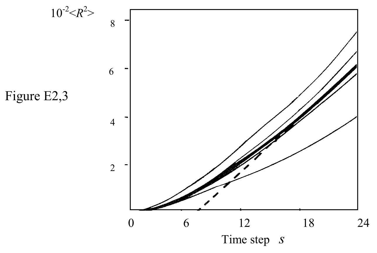
TYPICAL RESULTS : NOTE THE LARGE VARIATIONS IN THE VALUES OF $\langle R^2\rangle$

Time Number SZ - S-SR	SR = 261 $\langle R^2\rangle$	SR = 301 $\langle R^2\rangle$	SR = 334 $\langle R^2\rangle$	SR = 370 $\langle R^2\rangle$	AVERAGE $\langle R^2\rangle$
0	0	0	0	0	0
2	0.00088	0.00067	0.00091	0.00079	0.00081
4	0.00287	0.00276	0.00382	0.00298	0.00311
6	0.00523	0.00628	0.00858	0.00623	0.00658
8	0.00797	0.01101	0.01449	0.01039	0.01097
10	0.01143	0.01656	0.02095	0.01523	0.01604
12	0.01528	0.02235	0.02768	0.02022	0.02138
14	0.01874	0.02845	0.03453	0.02564	0.02684
16	0.02184	0.03539	0.04157	0.03160	0.03260
18	0.02526	0.04293	0.04902	0.03833	0.03889
20	0.02979	0.05080	0.05718	0.04532	0.04577
22	0.03538	0.05918	0.06605	0.0510	0.05303
24	0.04063	0.06784	0.07533	0.05569	0.05987

Оригинал в Архива: exp.pdf · официални решения: exp_sol.pdf