IPhO 1993, Експеримент — Задача 2. Magnetic Moments and Fields
Practical Competition — Experiment No. 2: Magnetic Moments and Fields · 14 юли 1993 г. · 10 т.
Внимание: Бележка към темата
The obtained archive booklet does not include a separate blank logarithmic plotting sheet or apparatus-specific envelope data. It includes complete apparatus diagrams and all worked sample measurements. Printed sample-table, uncertainty and unit discrepancies are preserved and identified in the solution.
Native practical competition cover and instructions
COUNTRY: ____________________
XXIV INTERNATIONAL PHYSICS OLYMPIAD
WILLIAMSBURG, VIRGINIA, U.S.A.
PRACTICAL COMPETITION — Experiment No. 2
July 14, 1993. Time available: 2.5 hours.
READ THIS FIRST! INSTRUCTIONS:
- Use only the pen provided, and only the equipment supplied.
- Use only the marked side of the paper.
- Write at the top of each page: the number of the problem; the number of the page of your report; the total number of pages in your report.
Example (for problem 1): 1 1/4; 1 2/4; 1 3/4; 1 4/4.
Условие
This experiment has two parts:
Part 1: To determine the absolute magnitude of the magnetic moment of a small cylindrical permanent magnet, contained in the envelope marked “X”. (A similar magnet, also needed for the experiment, is contained in the envelope marked “A”.)
Part 2: To investigate the magnetic field of a given axially symmetric distribution of magnets, contained in the envelope marked “B”.
In your experiments, you should make use of the following facts:
- The magnetic field produced by a dipole magnet at a point along its axis at distance from its center is parallel to that axis and of strength given by:
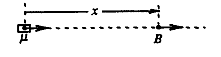
where is in Tesla [= N/(A m)], , is in m, and is in .
- The period of small torsional (angular) oscillations of a horizontal freely suspended magnet, such as a compass needle in the Earth's magnetic field, is given by:
where is the horizontal component of the net field at the magnet, and is the moment of inertia of the magnet about a vertical axis through its center.
Apparatus
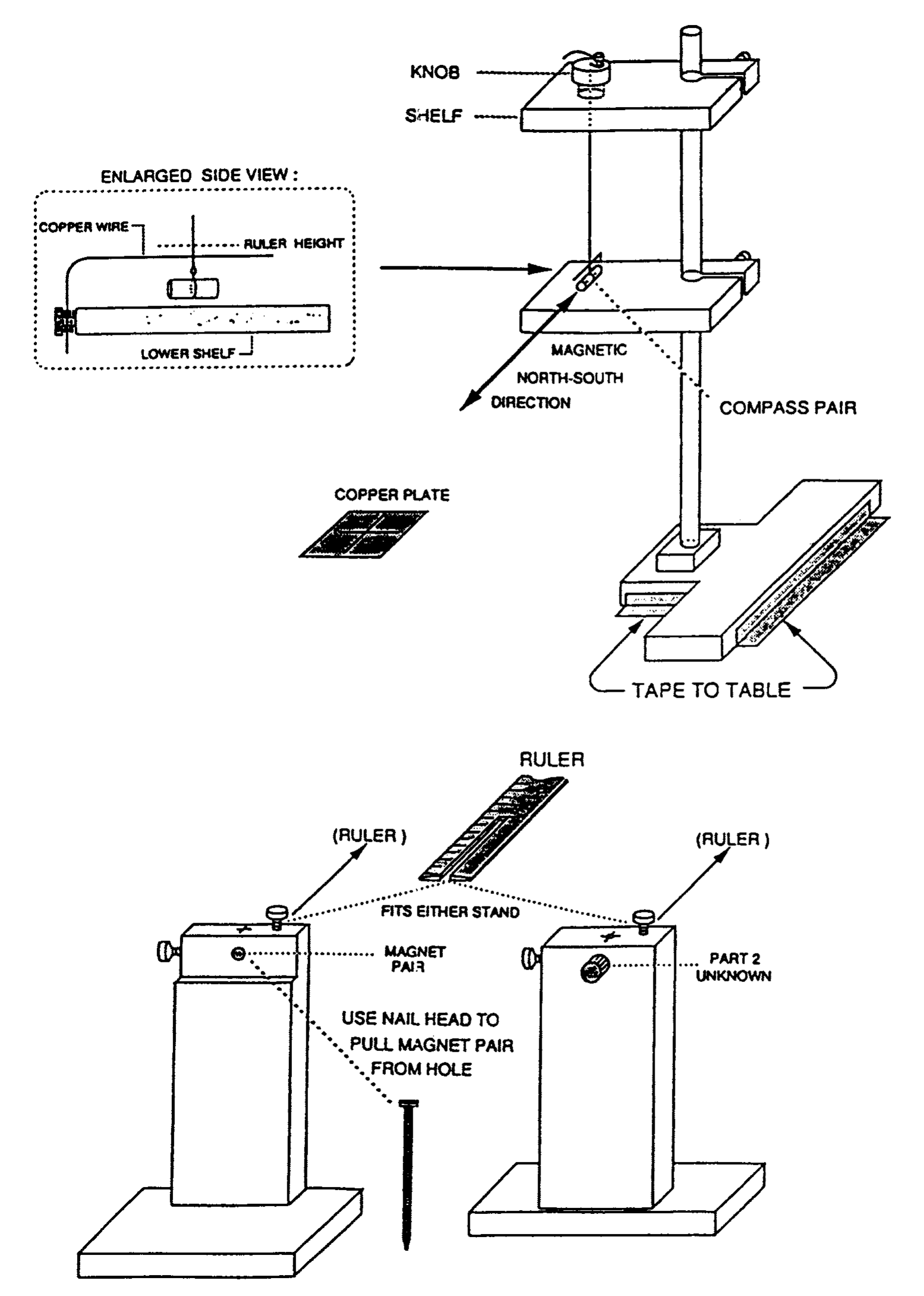
The apparatus is illustrated in the diagrams at the end. A thin thread is suspended from the upper of two shelves on a wooden stand. A magnet (“X” or “A”) can be attached to the bottom end of the thread. A copper plate can be placed on the lower shelf, just below the suspended magnet, to damp out its motion if desired. Two auxiliary wooden stands are provided. One of these serves as a holder for either “A” or “X” in Part 1; the other holds the magnet system B (used in Part 2). Distances between a suspended magnet and a magnet mounted in one of the auxiliary stands can be measured with a ruler mounted on that stand.
Warning: These magnets are extremely strong. Hold onto them tightly and be careful not to let them be pulled out of your fingers.
PART 1 The magnetic moment to be determined () is that of the pair of magnets in envelope X, labelled at the ends with a letter-number combination. Always keep this pair together. The moment of inertia of this pair has been calculated and written on envelope X. Envelope A contains another pair of magnets with north and south poles marked respectively with black and red spots. This pair is similar to the pair from envelope X, though its magnetic moment () cannot be assumed equal to .
A given pair of magnets can be “split” and placed around the bronze disk attached to the thread, forming a “compass” whose torsional oscillation period may be measured. (The value given on envelope X includes the effects of the bronze disk.)
One magnet-pair, centered in the hole in the wooden holder, can be used to influence the “compass” pair, possibly affecting its period and its angular equilibrium position. The angular position is best studied by placing the copper plate a few millimeters below the “compass” so as to provide electromagnetic damping. Please do not mark or write on the copper plate.
You will need to use more than one arrangement of the magnets. Draw clearly labelled diagrams showing each experimental arrangement used. Also, write equations to show how you will combine your different observations to obtain the value of .
Keep all magnets in the same horizontal plane. Note for the main stand that the top knob can be rotated, and the thread length adjusted. The position of each shelf can also be adjusted.
Practical Details (IMPORTANT!)
- COMPASS ASSEMBLY AND USE: Hold one magnet from a given pair between the thumb and forefinger of one hand. Center the bronze disk over one end. Then, carefully, and without pulling on the thread, slowly bring in the second magnet. This forms the compass pair (“X” or “A”). Also, avoid pulling on the thread in taking the compass apart. Warning: Rapid snapping of magnets or magnet pairs together can break the thread or chip the magnets. The tiny loop can be threaded again if thread breakage occurs. (Consult the organizers if necessary.)
- Study the torsional mode of oscillation. To prevent excitation of the “pendulum” mode, a small assembly made of copper wire is mounted on the lower shelf of the main stand. Rotate this assembly so that the horizontal piece is up against the thread at a point about 2 mm above where the thread is tied. With a slight additional rotation in the same direction, move the wire a few mm further. Warning: If this is not done, the two modes can “couple,” causing a periodic variation in the amplitude of the torsional oscillations, and affecting their period. Use the nail (see diagrams at end) to start the torsional oscillations in a controlled way.
- Keep magnetic or magnetizable objects stationary, and as far as possible from the experimental area. Consider such items as the nail, wrist watches, pens, etc. The table has some steel support parts; if you want to change the position of the apparatus, consider this fact.
Suggestions
(i) The torsion constant of the thread is quite small. It turns out that you can neglect its effect in the analysis provided the thread is reasonably long, e.g. around 15 cm.
(ii) You may notice that a given magnet pair does not hang horizontally. This is because of the vertical component of the Earth's field. The effect of this on the analysis is small and should be neglected. In other words, simply pretend that the magnet is horizontal.
(iii) We suggest that you postpone the error analysis for Part 1 until after you have made the measurements needed for Part 2.
(iv) You should not make any assumptions about the magnitude of the Earth's field. [6 т.]
PART 2 The aluminum tube (in envelope B) contains an axially symmetric distribution of magnets. The magnetic field along the axis, , of this assembly varies as a function of distance measured from the center of the tube according to the relation . Determine the exponent , with its approximate error. As sketched below, you should study the field on the side in the direction of the end marked with a black spot.

[4 т.]
WRITE YOUR SET-UP NUMBER ON YOUR REPORT. THIS IS THE LETTER-NUMBER COMBINATION PRINTED ON THE EQUIPMENT BOX AND ALSO ON THE MAGNET ENVELOPES LIKE THIS:
# ____________________
The obtained question does not print the numerical value written on the physical envelope X or an actual set-up letter-number combination. These apparatus-specific values are not supplied by the sample solution for another setup.
Apparatus diagrams
Решение
Part 1: Determination of μX — Basic Insight
Basic Insight
The idea which enables one to “see into” the problem is contained in the following remark: The oscillation period of a given suspended magnet depends on the product of its moment and the (horizontal component of) the Earth's field, while the extent to which that magnet can influence the direction of another magnet used as a compass depends on the ratio of those two quantities.
It follows that by making measurements of both types, both the unknown moment and the horizontal component of the Earth's field can be determined. We suspect that this idea goes historically back to Gauss.
First Solution: The “Turn-Around Method”
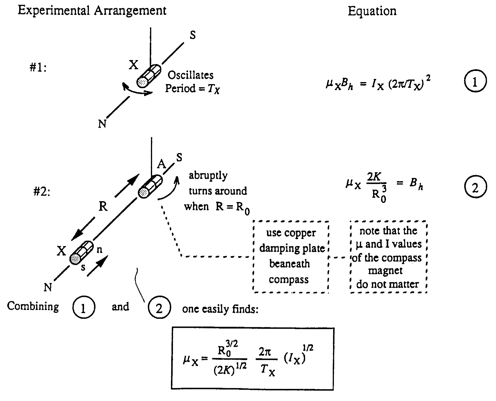
Experimental Arrangement #1: X oscillates with period .
Experimental Arrangement #2: A abruptly turns around when .
Use copper damping plate beneath compass. Note that the and values of the compass magnet do not matter.
Combining (1) and (2) one easily finds:
Second Solution: Dynamic Method with 3 Unknowns
The experience from our tests was that the “Turn-Around” method did not occur naturally to most students. They were much more comfortable with the idea of using one magnet to influence the period of another. Since the magnetic moments are not necessarily equal, it is clear that two measurements will no longer suffice. Our guess is that the following 3-measurement scheme will be the most common student choice.
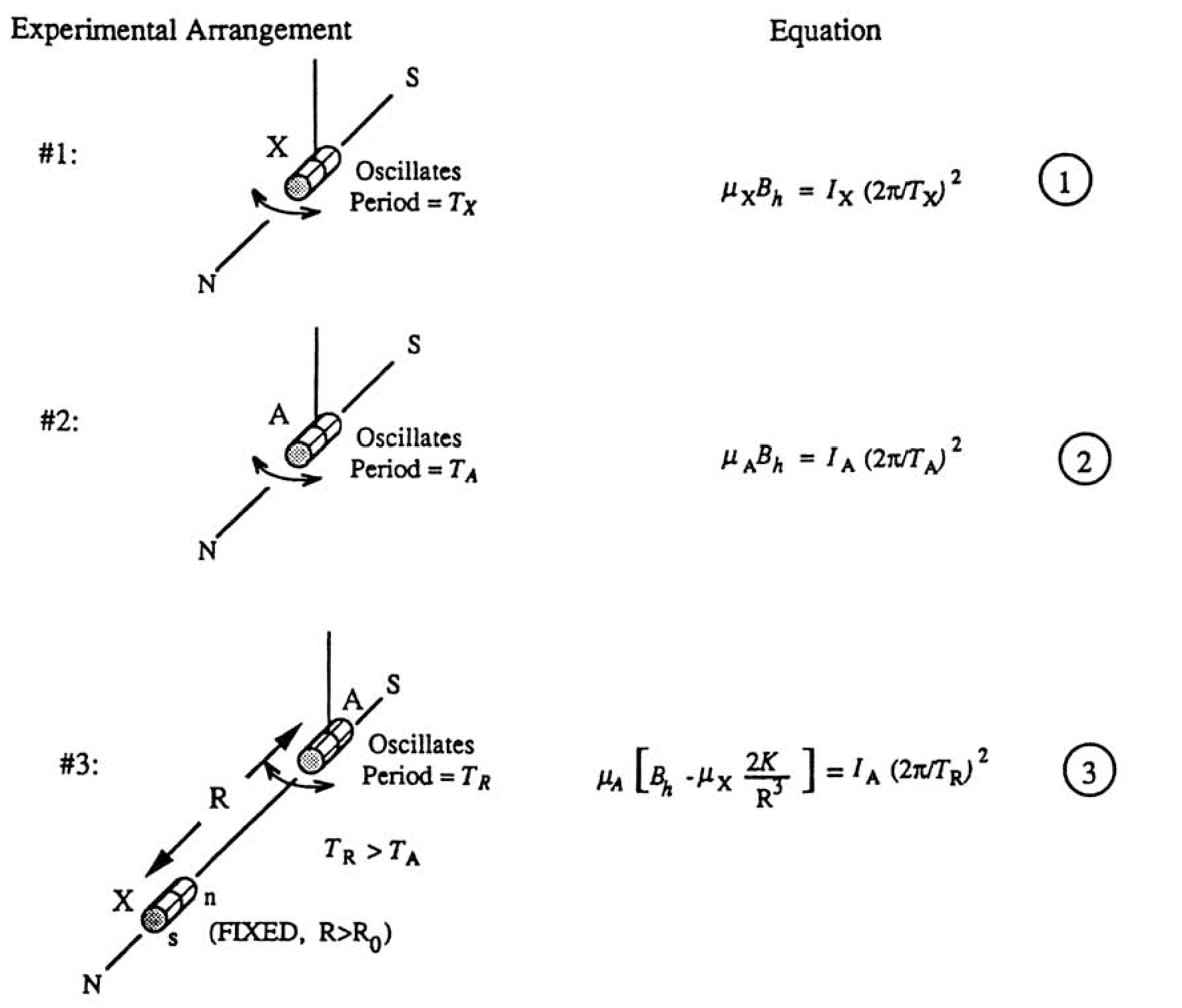
Arrangement #1: X oscillates with period .
Arrangement #2: A oscillates with period .
Arrangement #3: A oscillates with period ; X is fixed at .
Note that the X magnet (positioned at a distance which is somewhat larger than the turn-around distance ) is being used here to slow the oscillations of the A magnet on the compass.
One worries at first that there are actually 4 unknowns, since the inertial moment of A need not equal that of X. Inspection of equations (2) and (3) shows, however, that the ratio can be expressed in terms of experimentally known quantities. Since (1) gives the product , the calculational strategy is clear. One easily finds:
Alternatively, by reversing its poles, one can use the X magnet to speed-up the oscillations of the A magnet. Then, of course we have . In this case (which is formally equivalent to the first case, with a reversal of the sign of ), one finds:
Part 1 — Sample Experiment
The Dynamic Method just outlined was used (in the case where the X magnet was used to slow down the oscillations of the A magnet in Arrangement #3). In all cases 20 oscillations were timed. The distance was . The X moment of inertia was . Using the notation given previously, the data were as follows:
| Measurements in seconds | Four measured times | Arrangement |
|---|---|---|
| 10.83, 10.99, 10.91, 10.94 | #1 | |
| 10.95, 11.10, 11.01, 10.92 | #2 | |
| 21.70, 21.65, 21.78, 21.59 | #3 |
Using a pocket calculator (HP32S) to obtain the averages and statistical errors gives:
The “statistical errors” here are naively based on what the calculator gave for the estimated standard deviation around the sample mean. More carefully, one should divide this by the square root of the number of observations to give the estimated standard error of the sample mean. [Still more carefully, for such a small sample, one should apply the appropriate statistical correction factor.] For simplicity we will use the naively calculated results. This will suffice for our purposes.
Write (4) as , where
The expression for is identical for that for in the “turnaround method” when . This must be true, since in that case goes to infinity.
Numerically
then standard error propagation and reduction of the units give
which is a 1.5% uncertainty. For we find numerically:
The central value here is 0.862. One can easily use a pocket calculator to see the effects of the permitted statistical variations in each of the two places above. This shows that the effect of the numerator uncertainty is essentially , while that of the denominator is . Combining these statistically gives a net uncertainty in of 0.0026, so that the fractional uncertainty in is 0.0033. [An analysis of this by calculus is straightforward, but cumbersome.] Then the fractional uncertainty in is practically that in . We find:
The source prints A m on the product and A m² on the result; both unit forms are retained.
By way of comparison, measurement of the same magnet X using Fluxgate Magnetometry (at a distance of around 16 cm) gave .
Part 2: Distance Dependence of Field of “B” Unknown — Method I (Close Distances): Nulling of Transverse Static Deflection
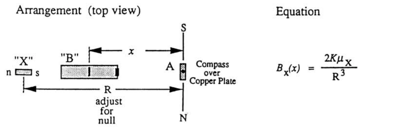
Arrangement (top view): A compass over copper plate; adjust for null.
Method II (Intermediate Distances): Differential 1/T² Technique
General Relation: ; = local (horiz.) field.
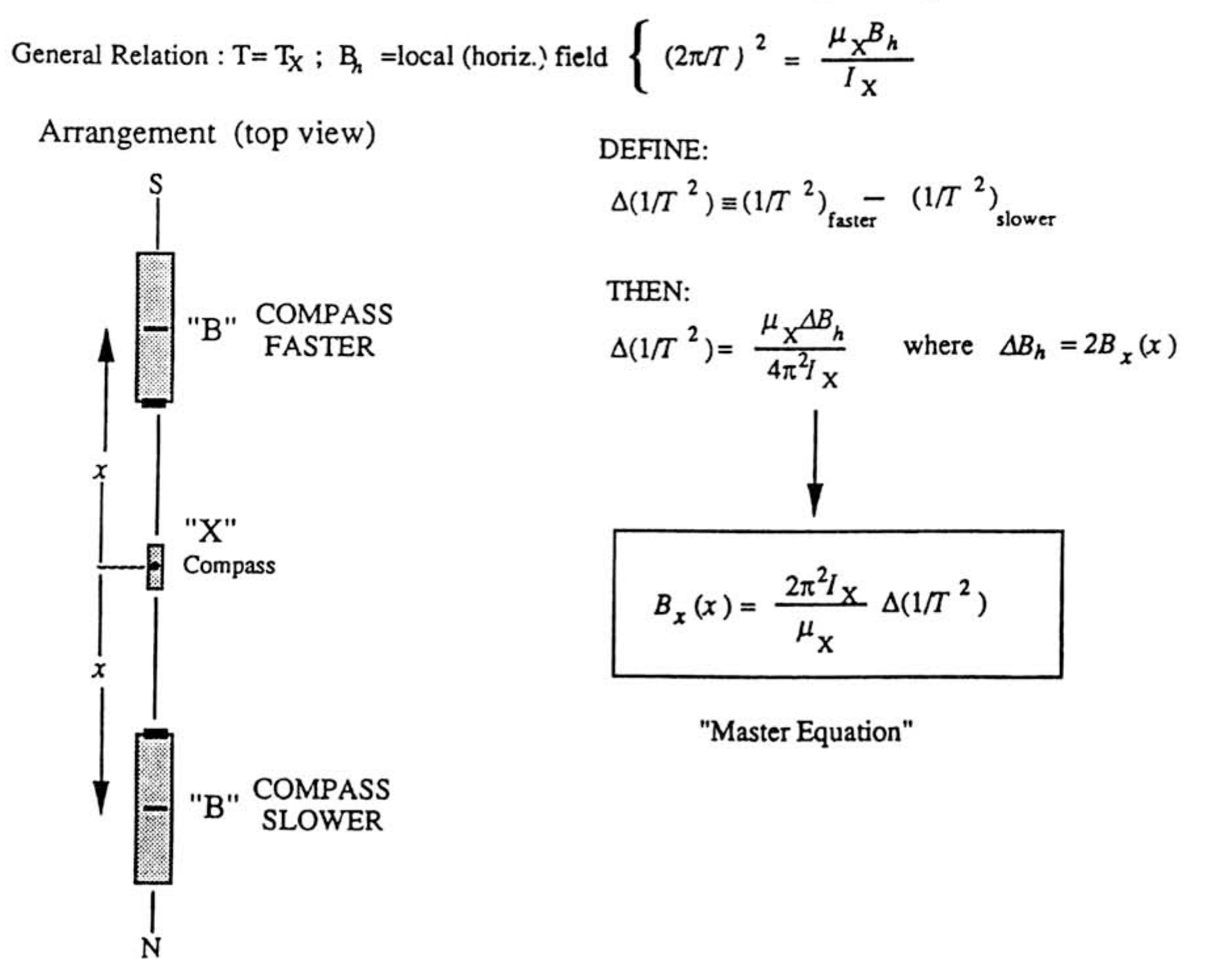
DEFINE:
THEN:
“Master Equation”
Method III (Large Distances): Differential 1/T² Technique with Partial “Bucking” of the Earth’s Field
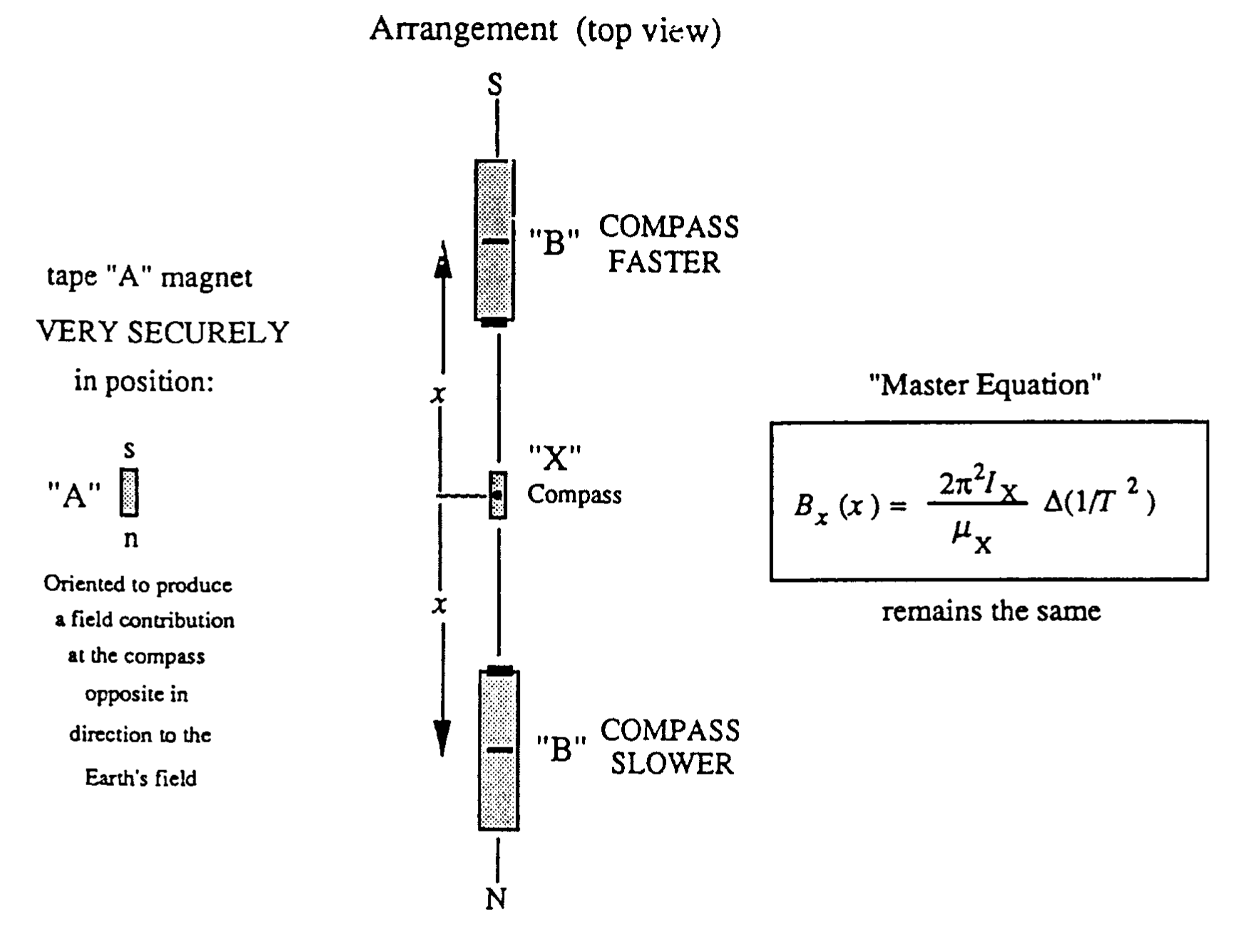
Tape “A” magnet VERY SECURELY in position: oriented to produce a field contribution at the compass opposite in direction to the Earth's field.
The “Master Equation” remains the same:
Use only partial buckout — (slow natural oscillations typically by a factor of 2).
In working at a given distance , must be constant (independent of the “bucking”).
Sample Experiment — Methods I and II
Method I
DATA TABLE FOR METHOD I
| Measured (m) | Measured (m) | Calculated ( T) | Standard error propagation | ||
|---|---|---|---|---|---|
| 493. | .031 | .065 | .072 | ||
| 294 | .019 | .085 | .087 | ||
| 149 | .039 | .071 | .081 | ||
| 79 | .074 | .059 | .095 |
The first native uncertainty is printed as ; it is retained, despite the smaller propagated uncertainty in the same row.
The uncertainty in includes the ruler reading error, together with the imprecision in locating the null position, the latter effect becoming predominant at larger . The uncertainty, together with the small uncertainty in , define the values listed in the 4th column.
Of course there are also the uncertainties in the values, which we could represent graphically by horizontal error bars. Since this is technically awkward, we choose instead to define an effective vertical uncertainty. Since it turns out that the log-log plot slope is about , a given fractional error in corresponds to 4 times as much in . These fractional errors have been tabulated in the 5th column. From this it is clear that we should take the effective as the square root of the sum of the squares of the contributions in columns 4 and 5. These values, listed in column 6, form the basis for the error bars used. Though we would certainly not expect a student to do this, we would expect him to be aware of the horizontal uncertainties.
Method II
:
| Data in seconds for 20 oscillations | Measured values | Pocket Calculator Results |
|---|---|---|
| 14.56, 14.50, 14.52, 14.58 | ||
| 11.32, 11.34, 11.31, 11.28 |
Sample Experiment — Method III
Introduced bucking magnet in transverse position to slow oscillations in Earth's Field to about 1.2 sec.
Master equation is still:
| Data in seconds for 20 oscillations | Measured values | Pocket Calculator Results |
|---|---|---|
| 27.90, 27.80, 27.78, 27.77 | ||
| 19.56, 19.66, 19.50, 19.64 |
The first unit in this native line is sec² and the result's unit is sec⁻²; both are retained.
| Data in seconds for 20 oscillations | Measured values | Pocket Calculator Results |
|---|---|---|
| 24.97, 24.97, 24.87 | ||
| 20.55, 20.46, 20.79, 20.65 |
| Data in seconds for 20 oscillations | Measured values | Pocket Calculator Results |
|---|---|---|
| 17.17, 17.15, 17.11, 17.10 | ||
| 16.01, 15.93, 15.91, 15.92 |
| Data in seconds for 20 oscillations | Measured values | Pocket Calculator Results |
|---|---|---|
| 23.80, 23.76, 23.70 | ||
| 22.27, 21.98, 21.86, 21.94 |
Sample Experiment — Tables, Power Law and Magnetometer Comparison
DATA TABLE FOR METHODS II and III
| (m) | Method | Calculated ( T) | Standard error propagation | ||
|---|---|---|---|---|---|
| II | 34.7 | .023 | .033 | .040 | |
| III | 14.8 | .024 | .027 | .036 | |
| III | 8.4 | .05 | .024 | .055 | |
| III | 6.0 | .13 | .021 | .13 | |
| III | 3.3 | .12 | .018 | .12 |
The equivalent vertical uncertainties have calculated as before and tabulated in the last column above. These give the error bars on the log-log plot shown on the next page. The three different methods are nicely consistent, and the whole data set well fits the power law indicated by the drawn line. When this is done on the regular log paper (as provided), the easiest way in this case to get the slope is to use a pocket calculator to find the ratio of the log of the vertical rise ratio to that of the horizontal run ratio for the possible lines consistent with the errors. Since the line has to drop vertically through three decades in total, this is roughly
The native denominator uncertainty is printed as .03; it is retained.
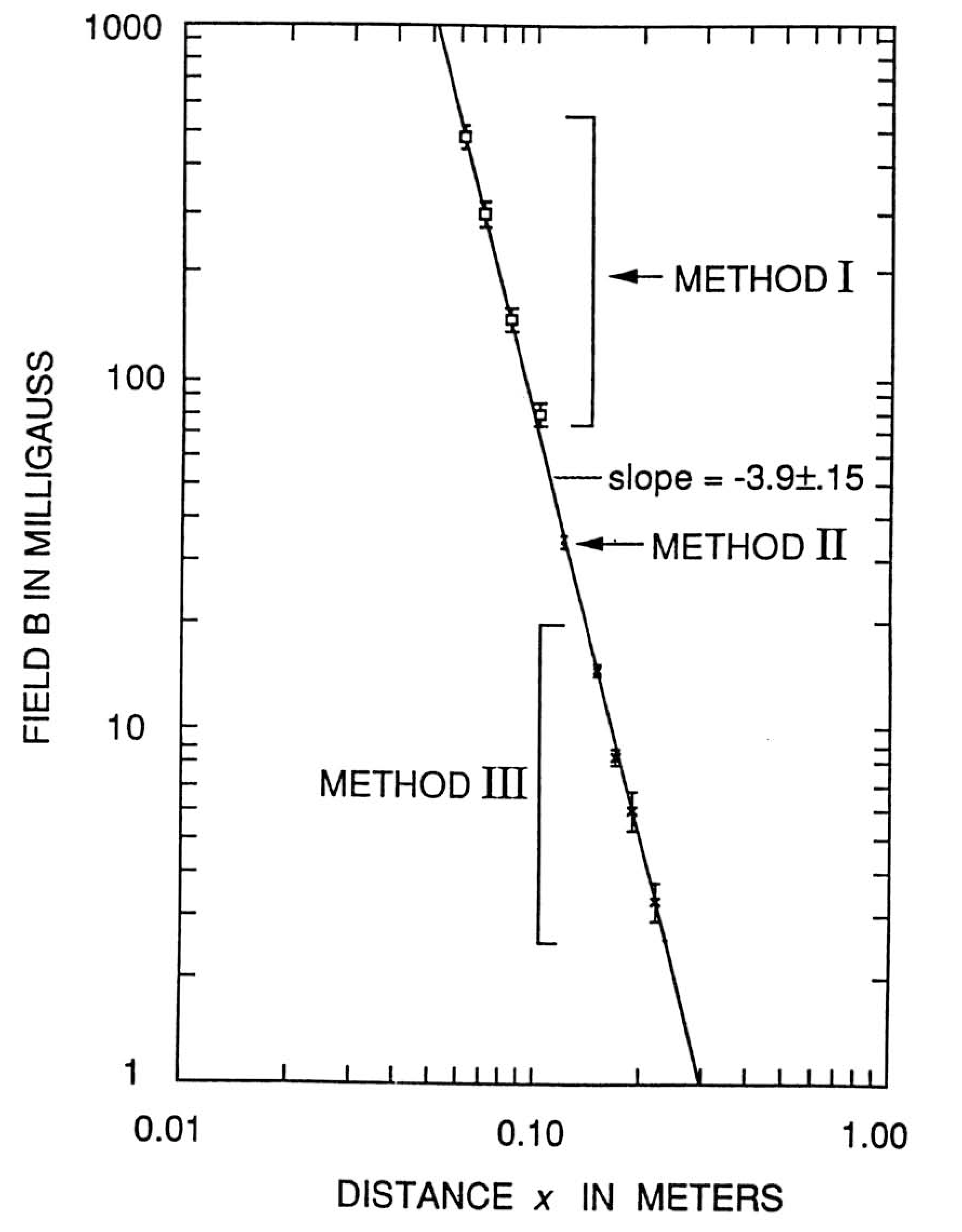
For this particular unknown, the fluxgate magnetometer data gave an effective exponent of over the range from 0.07 m to 0.22 m. A more detailed absolute comparison with those measurements is shown on the second graph. Here the drawn line corresponds to the actual magnetometer data. The student experiment is clearly doing an excellent job. Of particular interest is the next to the lowest point (). For this point, the “buckout” magnet had been moved out a little bit so that the natural compass period in the Earth's field was about 0.89 sec., which was close to the period of the “pendulum mode”. This was done deliberately to test the effectiveness of the copper wire “mode-decoupler”. The point at which is on the line was taken using the decoupler. The point at the same value which is almost a factor of 3 higher than the line was taken without the decoupler.
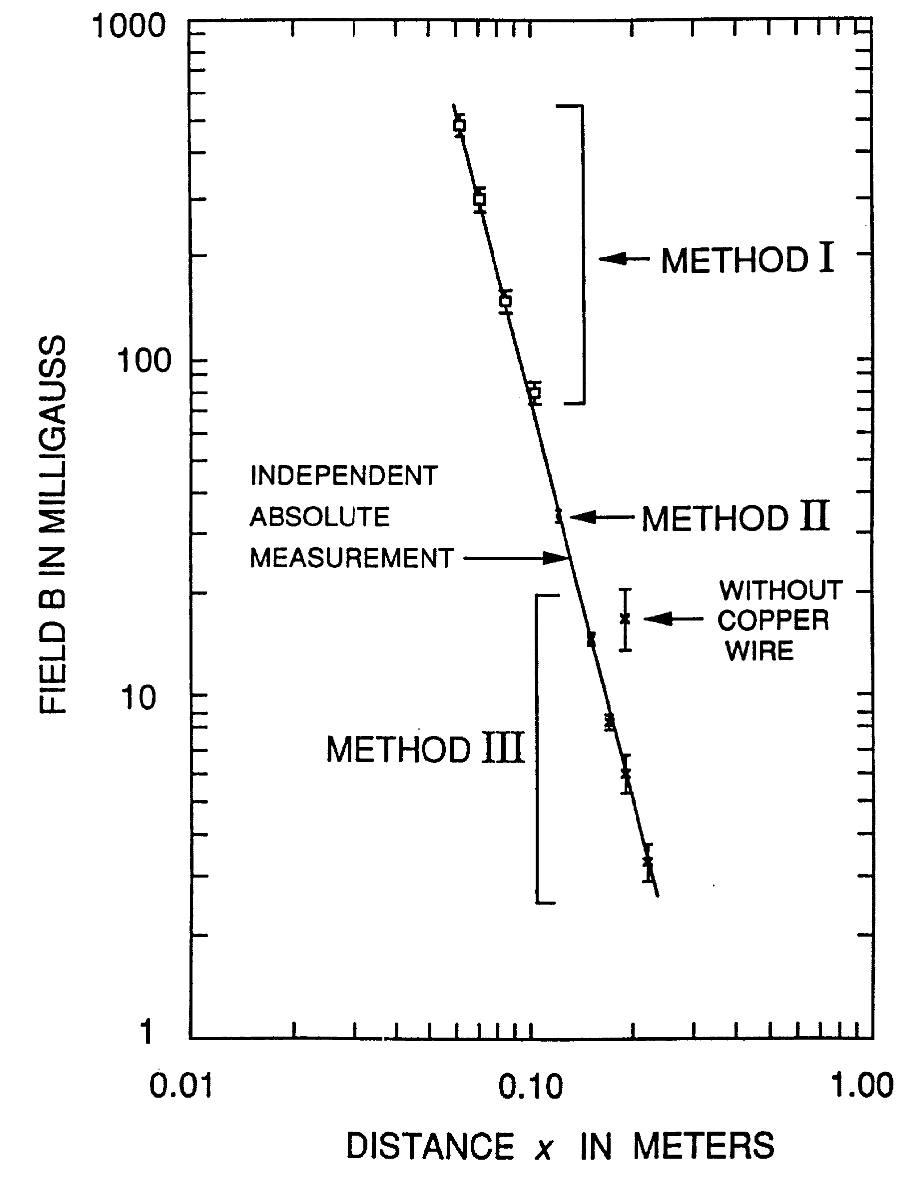
This shows that the decoupler is both effective and important. Without it, the “fast” and “slow” measurements are effected differently by the coupling to the pendulum mode. Then the small difference between them can be very poorly determined.
Experimental Problem 2: Grading Scheme
Part 1
| Points | Criterion |
|---|---|
| 2.5 | Show how is calculated, clearly labeled diagram |
| 1.5 | is correctly stated |
| 0–1 (sliding scale) | error analysis |
| 0–1 (sliding scale) | consistency with “correct” range |
Part 2
| Points | Criterion |
|---|---|
| 1.0 | A diagram of a technique that can be used |
| 1.0 | Correct measurements at 3 distances at least |
| 0–1 (sliding scale) | Accuracy of the result (correct value of ) |
| 0–1 (sliding scale) | Precision and error analysis |
Оригинал в Архива: ipho93.pdf · официални решения: ipho93.pdf