Съдържание

IPhO 2008, Експеримент — Задача 2. C. Task 2: Determining the efficiency of a solar cell under illumination of an incandescent lamp

Оригинал на условието (PDF)Съобщи за грешка

Всички материали от IPhO 2008

39th International Physics Olympiad - Hanoi - Vietnam - 2008 · Experimental Problem · DIFFERENTIAL THERMOMETRIC METHOD

Условие

1. Aim of the experiment

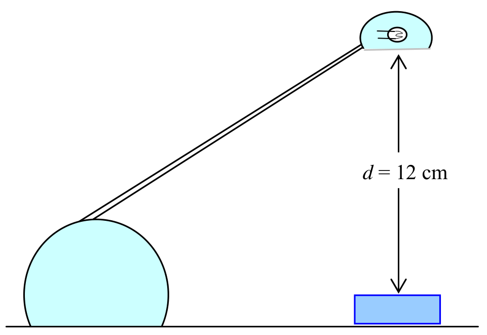
The aim of the experiment is to determine the efficiency of a solar cell under illumination of an incandescent lamp. Efficiency is defined as the ratio of the electrical power that the solar cell can supply to an external circuit, to the total radiant power received by the cell. The efficiency depends on the incident radiation spectrum. In this experiment the radiation incident to the cell is that of an incandescent halogen lamp. In order to determine the efficiency of the solar cell, we have to measure the irradiance $E$ at a point situated under the lamp, at a distance $d$ from the lamp along the vertical direction, and the maximum power $P_{\max}$ of the solar cell when it is placed at this point. In this experiment, $d$ = 12 cm (Figure 6). Irradiance $E$ can be defined by:

E=\Phi/S

Sketch of the halogen lamp: the round base on the left, an arm to the lamp head at the top right; a vertical arrow marked d = 12 cm runs from the lamp head down to a rectangular detector/solar cell on the table. — Figure 6. Using the halogen lamp as a light source

in which $\Phi$ is the radiant flux (radiant power), and $S$ is the area of the illuminated surface.

2. Apparatus and materials

The light source is a 20W halogen lamp.
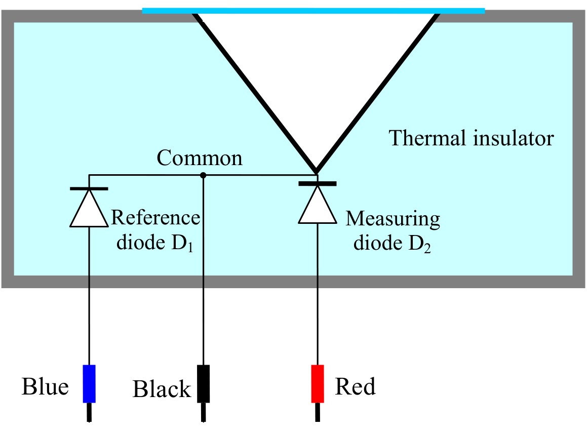
The radiation detector is a hollow cone made of copper, the inner surface of it is blackened with soot (Figure 7). The cone is incompletely thermally isolated from the surrounding. In this experiment, the detector is considered an ideal black body. To measure temperature, we use silicon diodes. The measuring diode is fixed to the radiation detector (D $_2$ in Figure 1 and Figure 7), so that its temperature equals that of the cone. The reference diode is placed on the inner side of the wall of the box containing the detector; its temperature equals that of the surrounding. The total heat capacity of the detector (the cone and the measuring diode) is $C=(0.69\pm0.02)\ \mathrm{J/K}$ . The detector is covered by a very thin polyethylene film; the radiation absorption and reflection of which can be neglected.
A circuit box as shown in Figure 2.
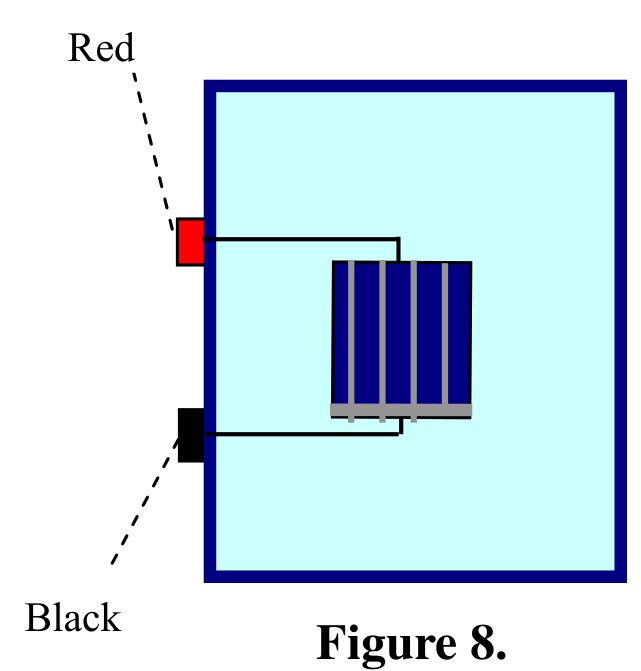
A piece of solar cell fixed on a plastic box (Figure 8). The area of the cell includes some metal connection strips. For the efficiency calculation these strips are considered parts of the cell.
Two digital multimeters. When used to measure the voltage, they have a very large internal resistance, which can be considered infinitely large. When we use them to measure the current, we cannot neglect their internal resistance. The voltage function of the multimeter has an error of ±2 on the last digit. The multimeters can also measure the room temperature.

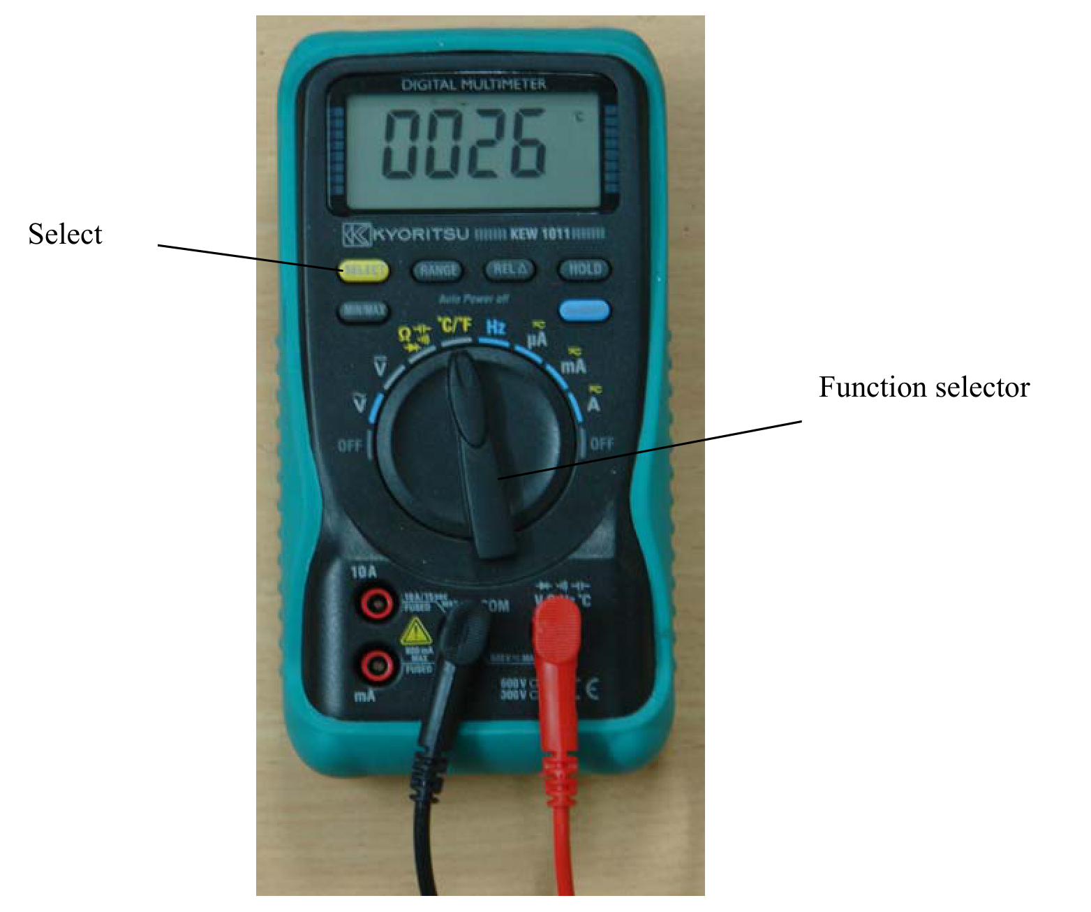
Cross-section of the radiation detector: a cone in a box filled with thermal insulator and covered by a film; the measuring diode D2 at the cone tip and the reference diode D1 on the wall share a common lead; leads end in Blue, Black and Red plugs. — Figure 7. Diagram of the radiation detector

Solar cell (dark striped rectangle) mounted on a light-blue plastic box, with a red socket labelled Red and a black socket labelled Black on the left side. — Figure 8. The solar cell

Note: to prevent the multimeter (see Figure 9) from going into the “Auto power off” function, turn the Function selector from OFF position to the desired function while pressing and holding the SELECT button.

A 9 V battery
A variable resistor.
A stop watch
A ruler with 1mm divisions
Electrical leads.
Graph papers.

3. Experiment

When the detector receives energy from radiation, it heats up. At the same time, the detector loses its heat by several mechanisms, such as thermal conduction, convection, radiation etc...Thus, the radiant energy received by detector in a time interval $dt$ is equal to the sum of the energy needed to increase the detector temperature and the energy transferred from the detector to the surrounding:

\Phi dt=CdT+dQ

where $C$ is the heat capacity of the detector and the diode, $dT$ - the temperature increase and $dQ$ - the heat loss.

When the temperature difference between the detector and the surrounding $\Delta T=T-T_0$ is small, we can consider that the heat $dQ$ transferred from the detector to the surrounding in the time interval $dt$ is approximately proportional to $\Delta T$ and $dt$ , that is $dQ=k\Delta Tdt$ , with $k$ being a factor having the dimension of W/K. Hence, assuming that $k$ is constant and $\Delta T$ is small, we have:

\Phi dt=CdT+k\Delta Tdt=Cd(\Delta T)+k\Delta Tdt

\frac{d(\Delta T)}{dt}+\frac{k}{C}\Delta T=\frac{\Phi}{C} \qquad (4)

The solution of this differential equation determines the variation of the temperature difference $\Delta T$ with time t, from the moment the detector begins to receive the light with a constant irradiation, assuming that at t=0, $\Delta T=0$

\Delta T(t)=\frac{\Phi}{k}\left(1-e^{-\frac{k}{C}t}\right) \qquad (5)

When the radiation is switched off, the mentioned above differential equation becomes

\frac{d(\Delta T)}{dt}+\frac{k}{C}\Delta T=0 \qquad (6)

and the temperature difference $\Delta T$ varies with the time according to the following formula:

\Delta T(t)=\Delta T(0)e^{-\frac{k}{C}t} \qquad (7)

where $\Delta T(0)$ is the temperature difference at $t=0$ (the moment when the measurement starts).

1 Determine the room temperature $T_0$ .

2. Compose an electric circuit comprising the diode sensors, the circuit box and the multimeters to measure the temperature of the detector.

In order to eliminate errors due to the warming up period of the instruments and devices, it is strongly recommended that the complete measurement circuit be switched on for about 5 minutes before starting real experiments.

2.1. Place the detector under the light source, at a distance of $d$ = 12 cm to the lamp. The lamp is off. Follow the variation of $\Delta V$ for about 2 minutes with sampling intervals of 10 s and determine the value of $\Delta V(T_0)$ in equation (3).

2.2. Switch the lamp on to illuminate the detector. Follow the variation of $\Delta V$ . Every 10-15 s, write down a value of $\Delta V$ in the table provided in the answer sheet. (Note: columns x and y of the table will be used later in section 4.). After 2 minutes, switch the lamp off.

2.3. Move the detector away from the lamp. Follow the variation of $\Delta V$ for about 2 minutes after that. Every 10-15 s, write down a value of $\Delta V$ in the table provided in the answer sheet. (Note: columns x and y of the table will be used later in section 3.).

Hints: As the detector has a thermal inertia, it is recommended not to use some data obtained immediately after the moment the detector begins to be illuminated or ceases to be illuminated.

3. Plot a graph in an x-y system of coordinates, with variables x and y chosen appropriately, in order to prove that after the lamp is switched off, equation (7) is satisfied.

3.1. Write down the expression for variables x and y.

3.2. Plot a graph of y versus x, called Graph 5.

3.3. From the graph, determine the value of $k$ .

4. Plot a graph in an x-y system of coordinates, with variables x and y chosen appropriately, in order to prove that when the detector is illuminated, equation (5) is satisfied.

4.1. Write down the expressions for variables x and y.

4.2. Plot a graph of y versus x, called Graph 6.

4.3. Determine the irradiance $E$ at the orifice of the detector.

5. Put the solar cell to the same place where the radiation detector was. Connect the solar cell to an appropriate electric circuit comprising the multimeters and a variable resistor which is used to change the load of the cell. Measure the current in the circuit and the voltage on the cell at different values of the resistor.

5.1. Draw a diagram of the circuit used in this experiment.

5.2. By rotating the knob of the variable resistor, you change the value of the load. Note the values of current $I$ and voltage $V$ at each position of the knob.

5.3. Plot a graph of the power of the cell, which supplies to the load, as a function of the current through the cell. This is Graph 7.

5.4. From the graph deduce the maximum power $P_{\max}$ of the cell and estimate its error.

5.5. Write down the expression for the efficiency of the cell that corresponds to the obtained maximum power. Calculate its value and error.

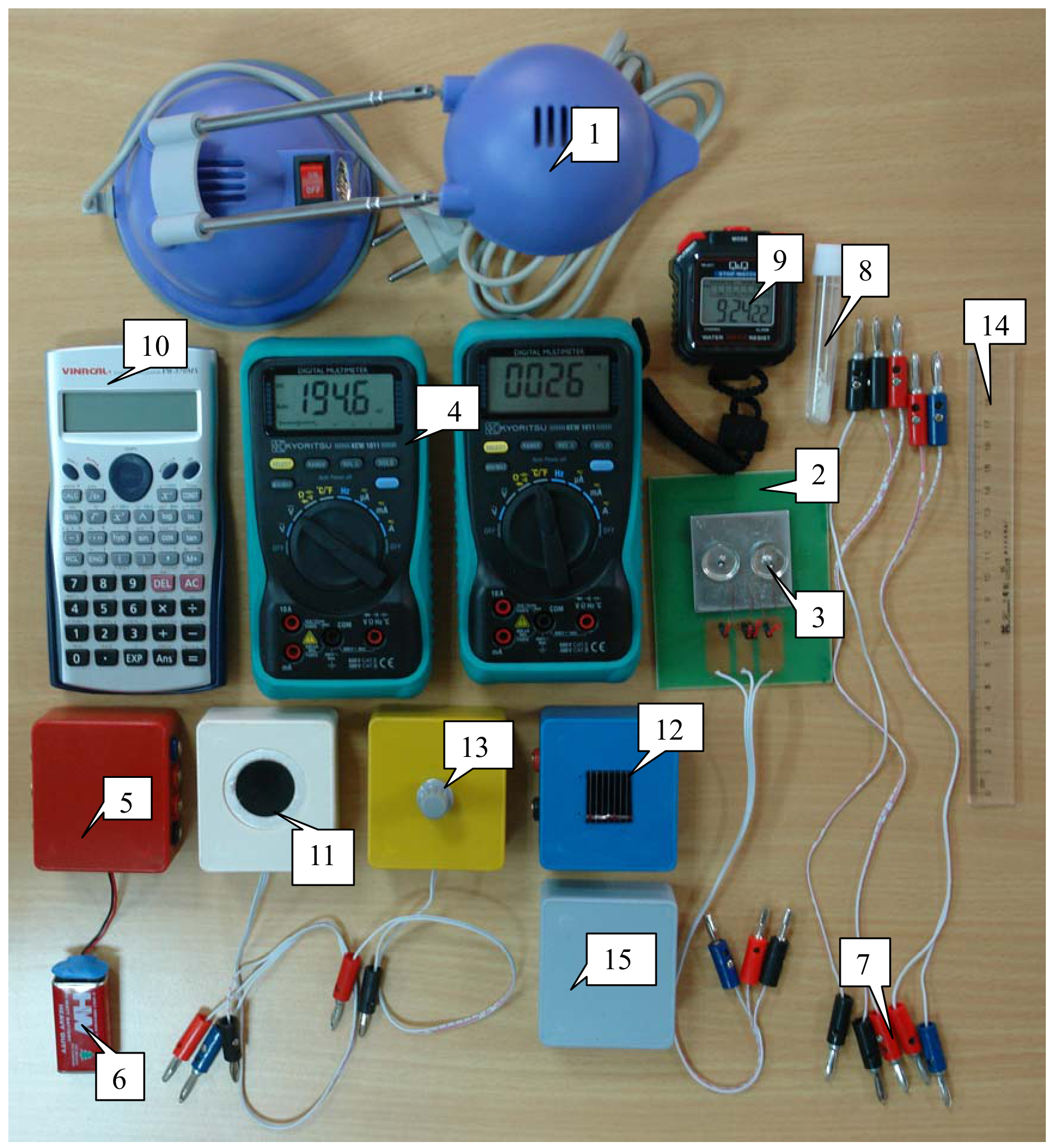
Contents of the experiment kit (see also Figure 10)

1	Halogen lamp 220 V/ 20 W	9	Stop watch
2	Dish holder	10	Calculator
3	Dish	11	Radiation detector
4	Multimeter	12	Solar cell
5	Circuit box	13	Variable resistor
6	9 V battery	14	Ruler
7	Electrical leads	15	Box used as a cover
8	Ampoule with substance to be measured

Photograph of a KYORITSU KEW 1011 digital multimeter showing 0026 on its display, with the SELECT button (label 'Select') and the rotary Function selector (label 'Function selector') indicated, and black and red test leads plugged in. — Figure 9. Digital multimeter

Photograph of the experiment kit with numbered labels 1–15: halogen lamp (1), dish holder (2), dish (3), multimeters (4), circuit box (5), 9 V battery (6), electrical leads (7), ampoule (8), stop watch (9), calculator (10), radiation detector (11), solar cell (12), variable resistor (13), ruler (14) and box used as a cover (15). — Figure 10. Contents of the experiment kit

Отговори

Решение

1.1. $T_0=26\pm1^{\circ}\mathrm{C}$

2.1. Measured data with the lamp off

t (s)	ΔV(T $_0$ ) (mV) (±0.2mV)
0	19.0
10	19.0
20	19.0
30	19.0
40	19.0
50	18.9
60	18.9
70	18.9
80	18.9
90	18.9
100	19.0
110	19.0
120	19.0

Values of ΔV(T $_0$ ) can be different from one experiment set to another. The acceptable values lie in between -40÷+40 mV.

2.2. Measured data with the lamp on

t (s)	ΔV (mV) (±0.2mV)
0	19.5
10	21.9
20	23.8
30	25.5
40	26.9
50	28.0
60	29.0
70	29.9
80	30.7
90	31.4
100	32.0
110	32.4
120	32.9

When illuminated (by the lamp) values of ΔV may change 10 ÷ 20 mV compared to the initial situation (lamp off).

2.3. Measured data after turning the lamp off

t (s)	ΔV (mV) (±0.2mV)
0	23.2
10	22.4
20	21.6
30	21.0
40	20.5
50	20.1
60	19.6
70	19.3
80	18.9
90	18.6
100	18.4
110	18.2
120	17.9

3. Plotting graph 5 and calculating k

3.1. $x=t$ ; $y=\ln\left[\Delta V(T_0)-\Delta V(t)\right]$

Note: other reasonable ways of writing expressions for x and y that also leads to a linear relationship using ln are also accepted.

3.2. Graph 5

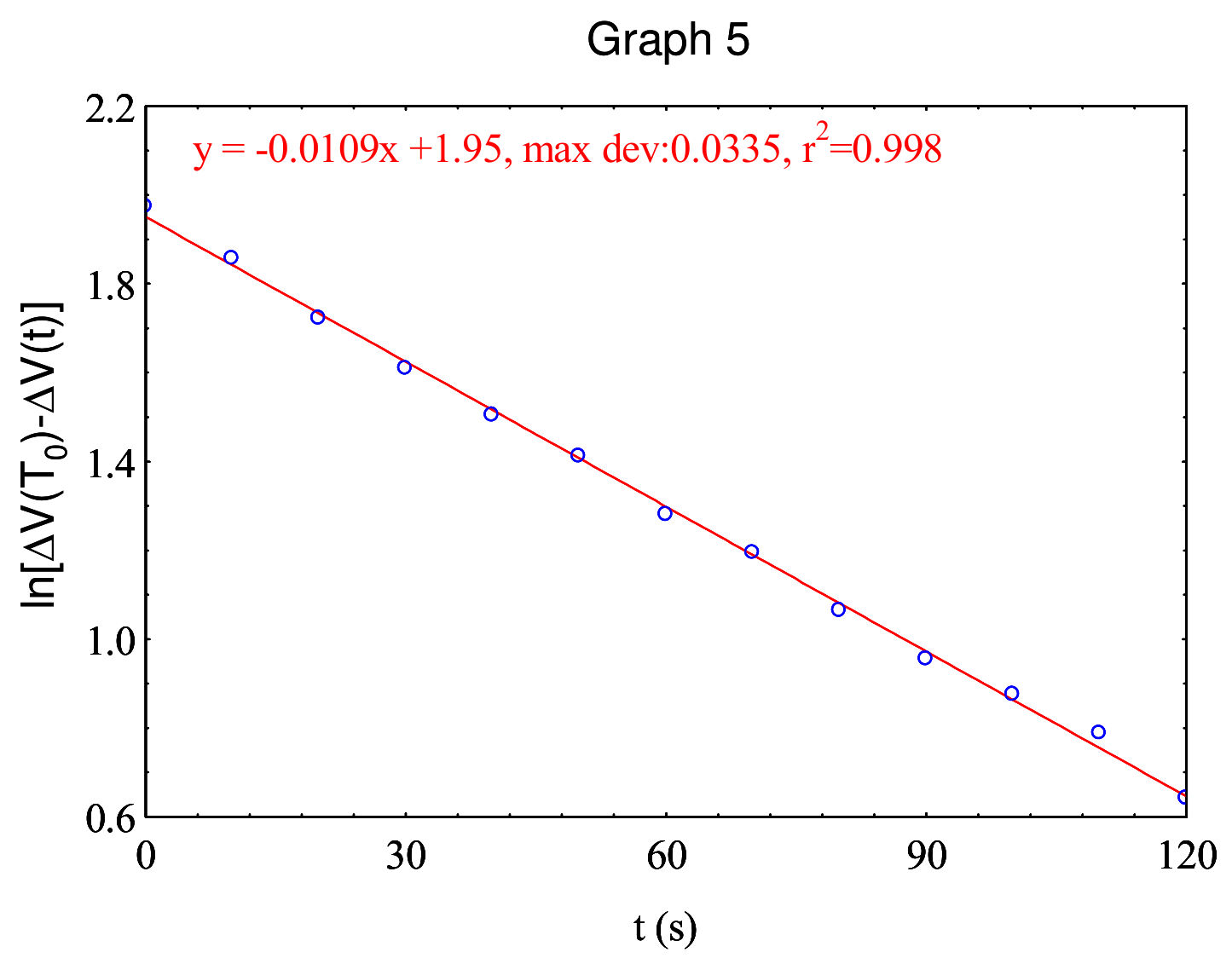
Graph 5: blue circles of ln[ΔV(T0)-ΔV(t)] (0.6–2.2) against t (s) (0–120) on a red fitted straight line, labelled 'y = -0.0109x +1.95, max dev:0.0335, r²=0.998'. — Graph 5

3.3. Calculating k: $\dfrac{k}{C}=0.0109\ \mathrm{s^{-1}}$ and $C=0.69\ \mathrm{J/K}$ , thus: $k=7.52\times10^{-3}\ \mathrm{W/K}$

Note: Error of k will be calculated in 5.5. Students are not asked to give error of k in this step. The acceptable value of k lies in between $6\times10^{-3}\div9\times10^{-3}\ \mathrm{W/K}$ depending on the experiment set.

4. Plotting Graph 6 and calculating E

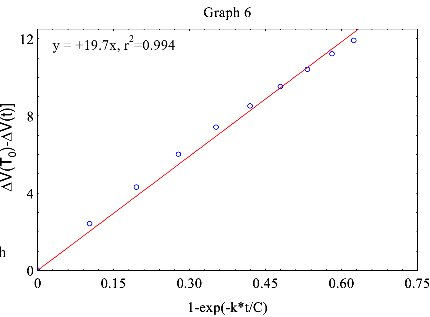
4.1. $x=\left[1-\exp\left(\dfrac{-kt}{C}\right)\right]$ ; $y=\left|\Delta V(T_0)-\Delta V(t)\right|$

Graph 6: blue circles of ΔV(T0)-ΔV(t) (0–12) against 1-exp(-k*t/C) (0–0.75) with a red straight line through the origin, labelled 'y = +19.7x, r²=0.994'. — Graph 6

4.2.

Graph 6 should be substantially linear, with the slope in between 15÷25 mV, depending on the experiment set.

4.3. From the slope of Graph 6 and the area of the detector orifice we obtain E = 140 W/m $^2$ . The area of the detector orifice is

S_{\mathrm{det}}=\pi R_{\mathrm{det}}^2=\pi\times(13\times10^{-3})^2=5.30\times10^{-4}\ \mathrm{m^2}\quad\text{with error: }\frac{\delta R_{\mathrm{det}}}{R_{\mathrm{det}}}=5\%

Error of E will be calculated in 5.5. Students are not asked to give error of E in this step. The acceptable value of E lies in between 120 ÷ 160 W/m $^2$ , depending on the experiment set.

5.1. Circuit diagram:

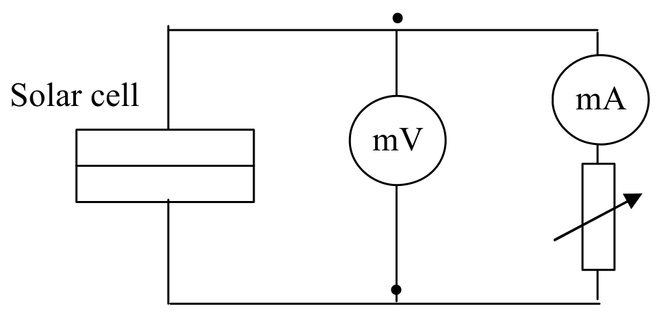
Circuit diagram: the solar cell connected in parallel with a voltmeter (mV) and with a branch containing an ammeter (mA) in series with a variable resistor. — Circuit diagram

5.2. Measurements of V and I

V (mV) (±0.3÷3mV)	I (mA) (±0.05÷0.1mA)	P (mW)
18.6 ±0.3	11.7	0.21
33.5	11.7	0.39
150	11.5	1.72
157	11.6	1.82
182 ±1	11.4	2.08
267	11.2	3.00
402 ±2	9.23	3.70
448	6.70	3.02
459	5.91	2.74
468	5.07	2.37
473 ±3	4.63	2.20
480	3.81	1.86
485	3.24	1.57
487	3.12	1.54
489	3.13	1.55

5.3.

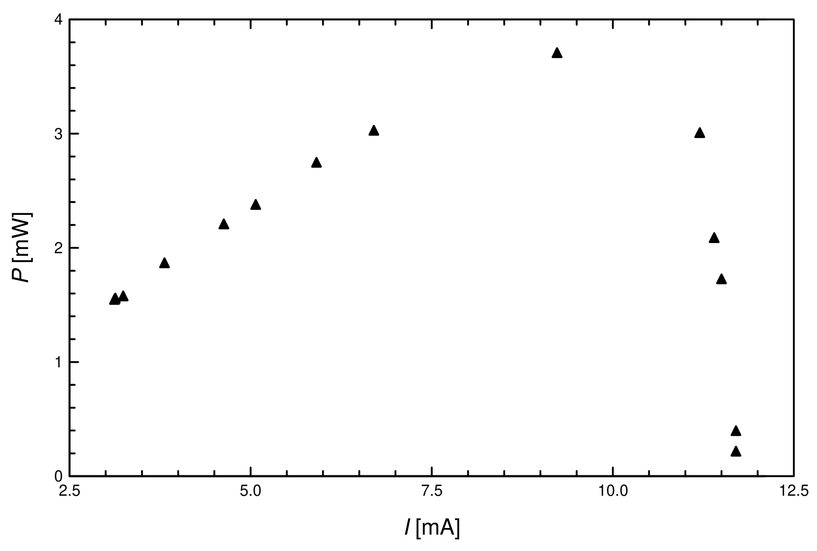
Graph 7: black triangles of P [mW] (0–4) against I [mA] (2.5–12.5); the power rises from about 1.5 mW at 3.1 mA to a maximum of about 3.7 mW near 9.2 mA and falls steeply to about 0.2 mW at 11.7 mA. — Graph 7

5.4. $P_{\max}=3.7\pm0.2\ \mathrm{mW}$

The acceptable value of $P_{\max}$ lies in between 3÷4.5 mW, depending on the experiment set.

5.5. Expression for the efficiency

S_{\mathrm{cell}}=19\times24\ \mathrm{mm^2}=450\times10^{-6}\ \mathrm{m^2}

Then $\eta_{\max}=\dfrac{P_{\max}}{E\times S_{\mathrm{cell}}}=0.058$

Error calculation:

\delta\eta_{\max}=\eta_{\max}\sqrt{\left(\frac{\delta P_{\max}}{P_{\max}}\right)^2+\left(\frac{\delta E}{E}\right)^2+\left(\frac{\delta S_{\mathrm{cell}}}{S_{\mathrm{cell}}}\right)^2}

, in which $S_{\mathrm{cell}}$ is the area of the solar cell.

$\dfrac{\delta P_{\max}}{P_{\max}}$ is estimated from Graph 7, typical value ≈ 6 %

$\dfrac{\delta S_{\mathrm{cell}}}{S_{\mathrm{cell}}}$ : error from the millimeter measurement (with the ruler), typical value ≈ 5 %

E is calculated from averaging the ratio (using Graph 6):

B=\frac{\Delta V(T_0)-\Delta V(t)}{1-\exp\left(-\frac{k}{C}t\right)}=\frac{E\pi R_{\mathrm{det}}^2\alpha}{k}

in which B is an intermediate variable, $R_{\mathrm{det}}$ is the radius of the detector orifice.

E=\frac{kB}{\pi R_{\mathrm{det}}^2\alpha}

Calculation of error of E:

\overline{\left(\frac{\delta E}{E}\right)}=\sqrt{\left(\frac{\delta k}{k}\right)^2+\left(\frac{\delta B}{B}\right)^2+4\left(\frac{\delta R_{\mathrm{det}}}{R_{\mathrm{det}}}\right)^2+\left(\frac{\delta\alpha}{\alpha}\right)^2}

k is calculated from the regression of:

\Delta T=\Delta T(0)\exp\left(-\frac{k}{C}t\right),\ \text{hence}\ \ln\Delta T=\ln\Delta T(0)-\frac{k}{C}t

We set $k/C=m$ then $k=mC$

From the regression, we can calculate the error of m:

\frac{\delta m}{m}\approx2(1-r)\approx0.2\%

\frac{\delta k}{k}=\sqrt{\left(\frac{\delta m}{m}\right)^2+\left(\frac{\delta C}{C}\right)^2}

We derive the expression for the error of $\eta_{\max}$ :

\delta\eta_{\max}=\eta_{\max}\sqrt{\left(\frac{\delta P_{\max}}{P_{\max}}\right)^2+\left(\frac{\delta S_{\mathrm{cell}}}{S_{\mathrm{cell}}}\right)^2+\left(\frac{\delta B}{B}\right)^2+4\left(\frac{\delta R_{\mathrm{det}}}{R_{\mathrm{det}}}\right)^2+\left(\frac{\delta m}{m}\right)^2+\left(\frac{\delta C}{C}\right)^2+\left(\frac{\delta\alpha}{\alpha}\right)^2}

Typical values for $\eta_{\max}$ and other constituent errors:

$\eta_{\max}\approx0.058$

$\dfrac{\delta P_{\max}}{P_{\max}}=5\%$ ; $\dfrac{\delta B}{B}\approx0.6\%$ ; $\dfrac{\delta m}{m}\approx0.2\%$ ; $\dfrac{\delta S_{\mathrm{cell}}}{S_{\mathrm{cell}}}\approx5\%$ ; $\dfrac{\delta R_{\mathrm{det}}}{R_{\mathrm{det}}}\approx5\%$ ;

$\dfrac{\delta C}{C}\approx3\%$ ; $\dfrac{\delta k}{k}\approx3\%$ ; $\dfrac{\delta E}{E}\approx10.5\%$ ; $\dfrac{\delta\alpha}{\alpha}\approx1.5\%$

Finally:

\frac{\delta\eta_{\max}}{\eta_{\max}}=12.7\%;\quad\delta\eta_{\max}\approx0.0074

and

\eta_{\max}=(5.8\pm0.8)\%

Note: if the student uses any other reasonable error method that leads to approximately the same result, it is also accepted.

Оригинал в Архива: exp.pdf · официални решения: exp_sol.pdf