Съдържание

Условие Introduction Forces between magnets Experimental setup (2

^{\mathrm{nd}}

problem)Tasks Решение

IPhO 2010, Експеримент — Задача 2. Experimental problem 2: Forces between magnets, concepts of stability and symmetry

Оригинал на условието (PDF)Съобщи за грешка

Всички материали от IPhO 2010

41st International Physics Olympiad – Experimental Competition, July 21st, 2010. Experimental problem 2 · 21 юли 2010 г. · 10 т.

Условие

There are two experimental problems. The setup on your table is used for both problems. You have 5 hours to complete the entire task (1&2).

Introduction

Electric current $I$ circulating in a loop of area $S$ creates a magnetic moment of magnitude $m = IS$ [see Fig. 1(a)]. A permanent magnet can be thought of as a collection of small magnetic moments of iron (Fe), each of which is analogous to the magnetic moment of a current loop. This (Ampère’s) model of a magnet is illustrated in Fig. 1(b). The total magnetic moment is a sum of all small magnetic moments, and it points from the south to the northern pole.

(a) A current loop of area S carrying current I, with magnetic field lines passing through it along the axis and looping around; (b) a cylindrical magnet drawn as a stack of small circular current loops with field lines running along its axis. — Figure 1. (a) Illustration of a current loop and the produced magnetic field. (b) Ampère’s model of a magnet as a collection of small current loops.

Forces between magnets

To calculate the force between two magnets is a nontrivial theoretical task. It is known that like poles of two magnets repel, and unlike poles attract. The force between two current loops depends on the strengths of the currents in them, their shape, and their mutual distance. If we reverse the current in one of the loops, the force between them will be of the same magnitude, but of the opposite direction.

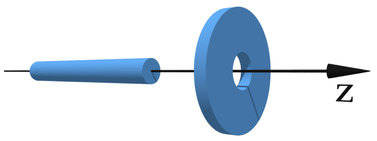
In this problem you experimentally investigate the forces between two magnets, the ring-magnet and the rod-magnet. We are interested in the geometry where the axes of symmetry of the two magnets coincide (see Fig. 2). The rod-magnet can move along the $z$ - axis from the left, through the ring-magnet, and then towards the right (see Fig. 2). Among other tasks, you will be asked to measure the force between the magnets as a function of $z$ . The origin $z = 0$ corresponds to the case when the centers of the magnets coincide.

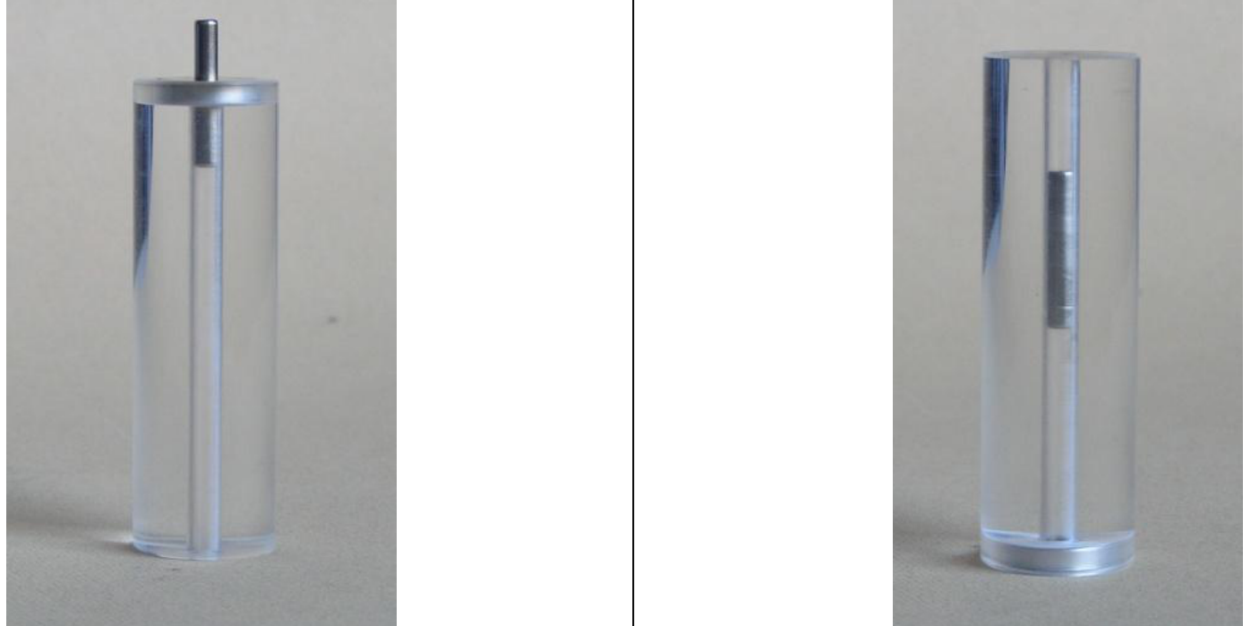
A blue rod-magnet on the left and a blue ring-magnet on the right, both centred on a common horizontal axis drawn as an arrow labelled z pointing to the right. — Figure 2. The rod- and the ring-magnet are aligned. The force between them changes as the rod-magnet moves along the z - axis.

To ensure motion of the rod-magnet along the axis of symmetry ( $z$ - axis), the ring-magnet is firmly embedded in a transparent cylinder, which has a narrow hole drilled along the $z$ - axis. The rod-magnet is thus constrained to move along the $z$ - axis through the hole (see Fig. 3). The magnetization of the magnets is along the $z$ - axis. The hole ensures radial stability of the magnets.

Two photographs of a transparent acrylic cylinder with a narrow axial hole; in the left photo the ring-magnet sits at the top with a thin rod sticking out, in the right photo the rod-magnet is visible inside the hole and the ring-magnet at the bottom. — Figure 3. Photo of two magnets and a transparent hollow cylinder; the rod-magnet moves through the cylinder’s hole.

Experimental setup (2 $^{\mathrm{nd}}$ problem)

The following items (to be used for the 2 $^{\mathrm{nd}}$ problem) are on your desk:

Press (together with a stone block); see separate instructions if needed
Scale (measures mass up to 5000 g, it has TARA function, see separate instructions if needed)
A transparent hollow cylinder with a ring-magnet embedded in its side.
One rod-magnet.
One narrow wooden stick (can be used to push the rod magnet out of the cylinder).

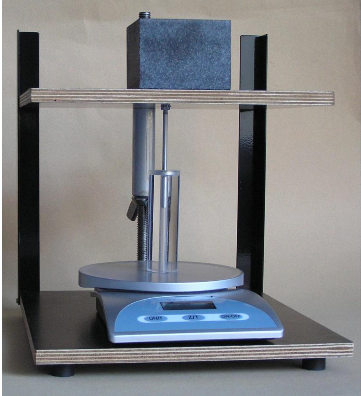
The setup is to be used as in Fig. 4 to measure the forces between the magnets. The upper plate of the press needs to be turned up-side-down in comparison to the first experimental problem. The narrow Aluminum rod is used to press the rod-magnet through the hollow cylinder. The scale measures the force (mass). The upper plate of the press can be moved downwards and upwards by using a wing nut. Important: The wing nut moves 2mm when rotated 360 degrees.

Photograph of the press: a wooden base plate with two black uprights, an upper plate carrying a stone block, a threaded rod with a wing nut, a thin aluminium rod pressing down into the transparent cylinder that stands on a digital kitchen scale with UNIT, Z/T and ON/OFF buttons. — Figure 4. Photograph of the setup, and the way it should be used for measuring the force between the magnets.

Tasks

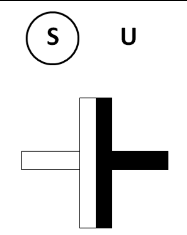
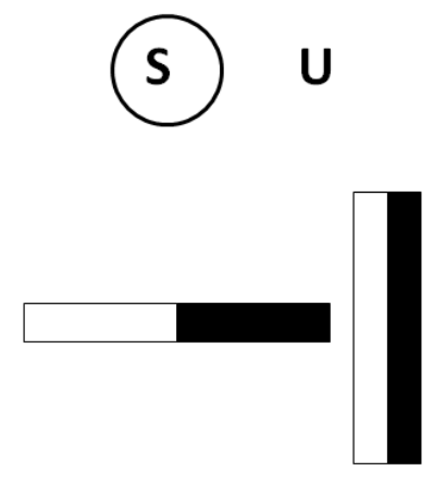
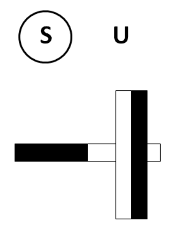
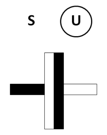
1. Determine qualitatively all equilibrium positions between the two magnets, assuming that the $z$ - axis is positioned horizontally as in Fig. 2 , and draw them in the answer sheet. Label the equilibrium positions as stable (S)/unstable (U), and denote the like poles by shading, as indicated for one stable position in the answer sheet. You can do this Task by using your hands and a wooden stick. (2.5 points)

2. By using the experimental setup measure the force between the two magnets as a function of the $z$ - coordinate. Let the positive direction of the $z$ - axis point into the transparent cylinder (the force is positive if it points in the positive direction). For the configuration when the magnetic moments are parallel, denote the magnetic force by $F_{\uparrow\uparrow}(z)$ , and when they are anti-parallel, denote the magnetic force by $F_{\uparrow\downarrow}(z)$ . Important: Neglect the mass of the rod-magnet (i.e., neglect gravity), and utilize the symmetries of the forces between magnets to measure different parts of the curves. If you find any symmetry in the forces, write them in the answer sheets. Write the measurements on the answer sheets; beside every table schematically draw the configuration of magnets corresponding to each table (an example is given). (3.0 points)

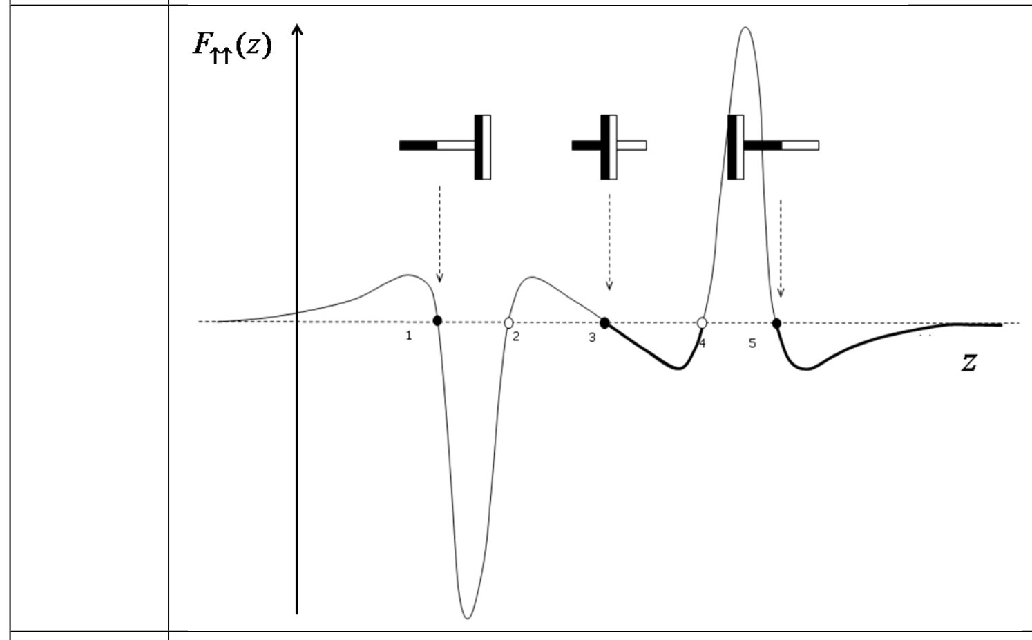
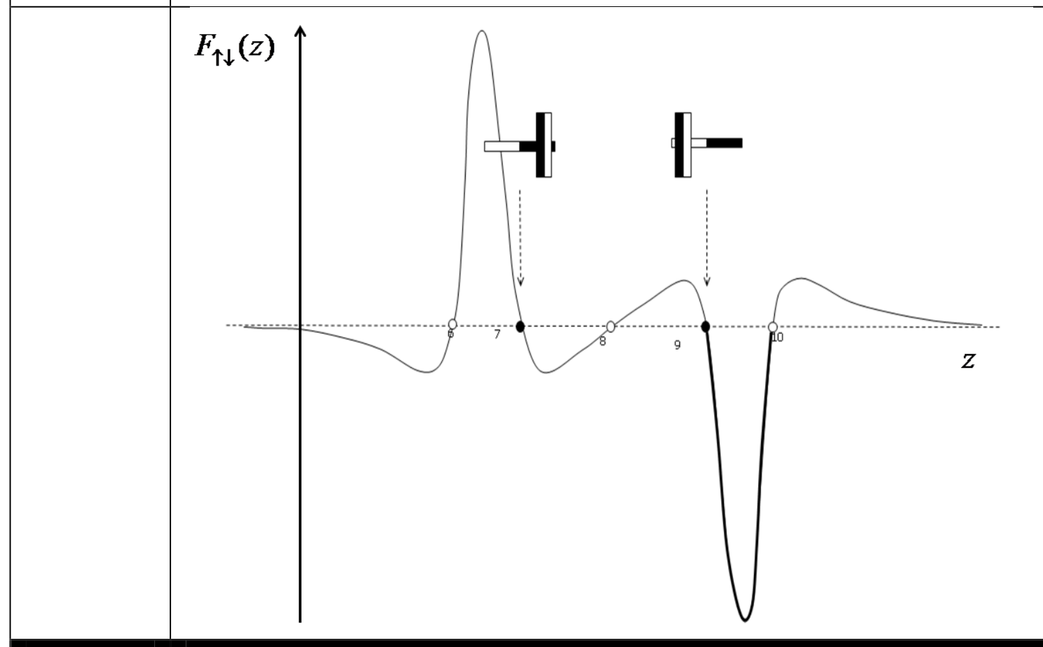
3. By using the measurements from Task 2, use the millimeter paper to plot in detail the functional dependence $F_{\uparrow\uparrow}(z)$ for $z > 0$ . Plot schematically the shapes of the curves $F_{\uparrow\uparrow}(z)$ and $F_{\uparrow\downarrow}(z)$ (along the positive and the negative $z$ - axis). On each schematic graph denote the positions of the stable equilibrium points, and sketch the corresponding configuration of magnets (as in Task 1). (4.0 points)

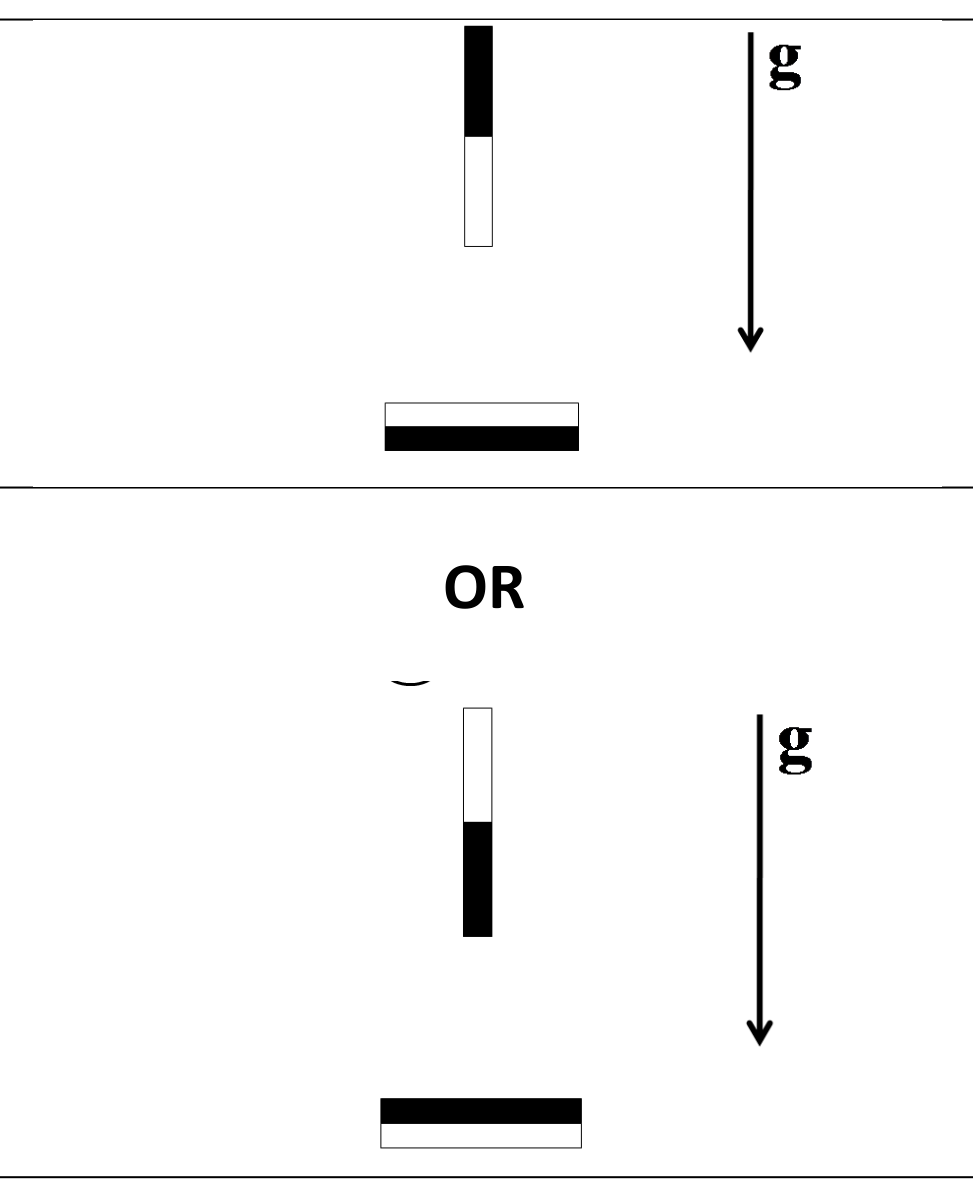
4. If we do not neglect the mass of the rod magnet, are there any qualitatively new stable equilibrium positions created when the $z$ - axis is positioned vertically? If so, plot them on the answer sheet as in Task 1. (0.5 points)

Решение

Task 1 — Points

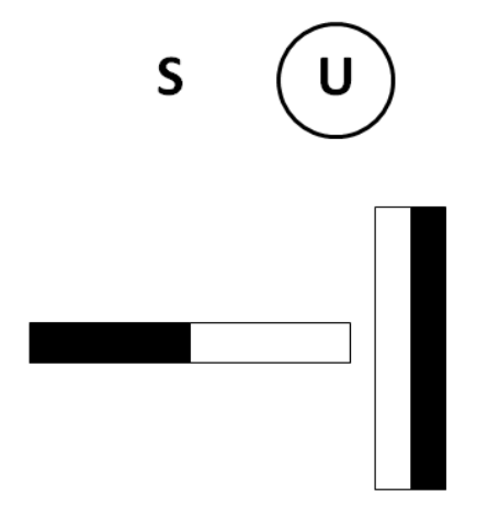
Six equilibrium configurations are drawn (figures below); in each, the correct label, S or U, is circled.

S (circled) — 0.25
S (circled) — 0.45
S (circled) — 0.45
U (circled) — 0.45
U (circled) — 0.45
U (circled) — 0.45

Task 2 — Points

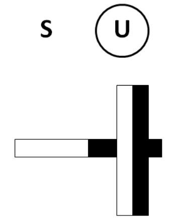
Task 1, configuration 5 (0.45 points): letters S and U (circled) above a sketch of the rod-magnet (black on the left, white on the right) to the left of the ring-magnet (white left, black right).

Task 1, configuration 6 (0.45 points): letters S and U (circled) above a sketch of the rod-magnet (white on the left, black on the right) inserted from the left just through the ring-magnet (white left, black right).

Symmetries that should be utilized in the measurements: 0,6

F_{\uparrow\downarrow}(z) = -F_{\uparrow\downarrow}(-z)

F_{\uparrow\downarrow}(z) = -F_{\uparrow\uparrow}(z)

From the two above one gets also $F_{\uparrow\uparrow}(z) = -F_{\uparrow\uparrow}(-z)$

By using the setup as it is, the whole curve can be measured by starting the measurements from three stable equilibrium points; the equilibrium point (z0) can be measured also by using the setup. 0,8

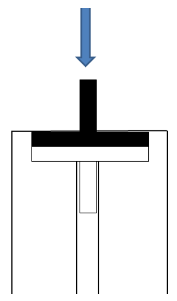
Task 2, first measurement configuration: a blue arrow pressing down on a vertical rod; the ring-magnet (black over white) lies across the top of the transparent cylinder, with the rod-magnet in the hole directly beneath it.

Configuration: (figure)

Measurements:

z0=0mm	m [g]	Δz [mm]
	0	0
	31	1
	55	2
	75	3
	97	4
	119	5
	140	6
	158	7
	171	8
	170	9
	118	10
	85	10,25
	50	10,5
	10	10,75

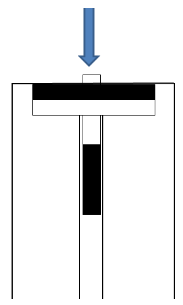
Task 2, second measurement configuration: a blue arrow pressing down; the ring-magnet (black over white) at the top of the cylinder and a black rod-magnet lower down in the hole, below a white segment.

0,8

Configuration: (figure)

Measurements:

z0=10.8mm	m [g]	Δz [mm]
	0	0
	233	1
	538	2
	927	3
	996	3,5
	1124	4
	1154	4,5
	1213	5
	1212	5,5
	1120	6
	873	6,5
	284	7
	36	7,5

0,8

Configuration: (figure)

Measurements:

z0=18.6mm	m [g]	Δz [mm]
	0	0
	116	1
	170	2
	186	3
	184	4
	169	5
	150	6
	116	8
	89	10
	67	12
	53	14
	36	16
	27	18
	23	20
	14	22
	9	24
	5	26
	3	28

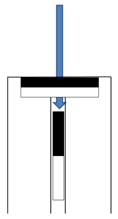
Task 2, third measurement configuration: a long blue arrow passing through the ring-magnet (black over white) at the top of the cylinder and pushing down on the rod-magnet (black top half, white bottom half) inside the hole.

Task 3 — Points

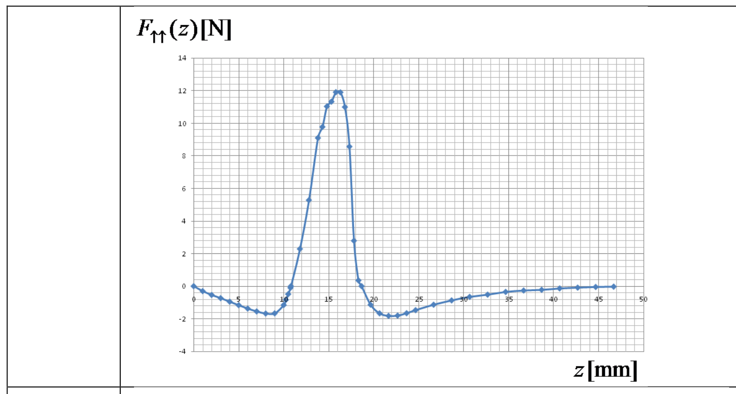
Due to symmetry, it is sufficient to plot e.g., the following graph in detail: 2

(detailed graph of $F_{\uparrow\uparrow}(z)$ [N] versus $z$ [mm])

Schematic graph of $F_{\uparrow\uparrow}(z)$ with the stable equilibrium configurations: 1

Schematic graph of $F_{\uparrow\downarrow}(z)$ with the stable equilibrium configurations: 1

Task 4 — Points

Two configurations are drawn (figure): 0,5

Total: 10.0

Task 1, configuration 1 (0.25 points): letters S (circled) and U above a sketch of the rod-magnet passing through the centre of the ring-magnet; the left half of each magnet is white and the right half black (like poles shaded).

Task 1, configuration 2 (0.45 points): letters S (circled) and U above a sketch of the rod-magnet to the left of the ring-magnet, rod white on the left and black on the right, ring white on the left and black on the right.

Task 1, configuration 3 (0.45 points): letters S (circled) and U above a sketch of the rod-magnet (black on the left, white on the right) partly inserted from the left through the ring-magnet (white left, black right).

Task 1, configuration 4 (0.45 points): letters S and U (circled) above a sketch of the rod-magnet (black on the left, white on the right) centred in the ring-magnet (white left, black right).

Task 3, detailed graph of F↑↑(z) [N] versus z [mm] on millimetre grid, z from 0 to 50 and F from −4 to 14: the force dips slightly negative to about −1.7 near z ≈ 9, rises sharply to a peak of about 12 near z ≈ 16, falls to about −1.8 near z ≈ 22 and then approaches zero.

Task 3, schematic graph of F↑↑(z) along the whole z axis with zero crossings numbered 1 to 5; filled dots mark stable equilibria at 1, 3 and 5 and open dots unstable ones at 2 and 4; small magnet sketches with dashed arrows show the configurations at the stable points; a deep negative trough lies between 1 and 2 and a high positive peak between 4 and 5.

Task 3, schematic graph of F↑↓(z) with zero crossings numbered 6 to 10; filled dots mark stable equilibria at 7 and 9, open dots unstable ones at 6, 8 and 10; two magnet sketches with dashed arrows show the stable configurations; a high positive peak lies between 6 and 7 and a deep negative trough between 9 and 10.

Task 4: two vertical configurations separated by the word OR, each with a downward arrow labelled g: a rod-magnet hovering above a ring-magnet, the upper one with the rod black on top and white below over a ring white on top and black below, the lower one with the rod white on top and black below over a ring black on top and white below.

Оригинал в Архива: exp2.pdf · официални решения: exp2_sol.pdf

z0=18.6mm	m [g]	Δz [mm]
	0	0
	116	1
	170	2
	186	3
	184	4
	169	5
	150	6
	116	8
	89	10
	67	12
	53	14
	36	16
	27	18
	23	20
	14	22
	9	24
	5	26
	3	28

z0=18.6mm	m [g]	Δz [mm]
	0	0
	116	1
	170	2
	186	3
	184	4
	169	5
	150	6
	116	8
	89	10
	67	12
	53	14
	36	16
	27	18
	23	20
	14	22
	9	24
	5	26
	3	28

Съдържание

IPhO 2010, Експеримент — Задача 2. Experimental problem 2: Forces between magnets, concepts of stability and symmetry

Условие

Introduction

Forces between magnets

Experimental setup (2nd^{\mathrm{nd}}nd problem)

Tasks

Решение

Experimental setup (2 $^{\mathrm{nd}}$ problem)

z0=18.6mm	m [g]	Δz [mm]
	0	0
	116	1
	170	2
	186	3
	184	4
	169	5
	150	6
	116	8
	89	10
	67	12
	53	14
	36	16
	27	18
	23	20
	14	22
	9	24
	5	26
	3	28