Съдържание
УсловиеPart A. Four-point-probe (4PP) measurements (1,2 т.)Part B. Sheet resistivity (0,3 т.)Part C. Measurements for different sample dimensions (3,2 т.)Part D. Geometrical correction factor: scaling law (1,9 т.)Part E. The silicon wafer and the van der Pauw-method (3,4 т.)ОтговориРешениеIPhO 2016, Експеримент — Задача 1. Electrical conductivity in two dimensions
IPhO 2016 International Physics Olympiad Switzerland Liechtenstein — Experiment, English (Official), Q1 · 10 т.
Условие
Please read the general instructions in the separate envelope before you start this problem.
Introduction
In the quest to develop next generation devices based on semi-conductor technology like computer chips or solar cells, researchers are looking for materials which exhibit outstanding transport properties, e.g. low electrical resistivity. Measurements of these properties are carried out using samples of finite size, contacts with finite contact resistance and in a special geometry. These effects have to be taken into account in order to extract the true material properties. Moreover, a thin film of the material may behave differently than bulk material.
In this task, we will investigate the measurement of electrical properties. We will use two different definitions:
- Resistance : The resistance is the electrical property of a sample or device. It is the quantity which we actually measure on a specific sample with given dimensions.
- Resistivity : The resistivity is the material property which determines the resistance. It depends on the material itself and on external parameters like the temperature, but it does not depend on the geometry of the sample.
In particular, we will measure the so-called sheet resistivity. This is the resistivity divided by the thickness of the very thin sheet.
We will explore the influence of the following parameters on the measurement of the electrical resistance of thin layers of material:
- the measurement circuitry,
- the measurement geometry,
- and the sample dimensions.
A sheet of conductive paper and a metal coated silicon wafer will serve as samples.
List of materials
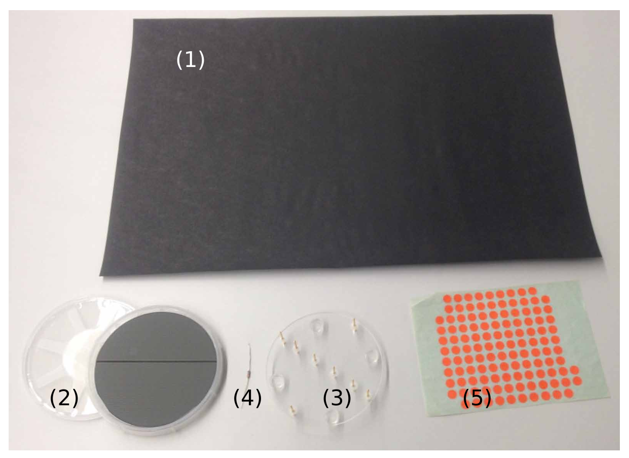
- Graphite coated conductive paper
- A silicon wafer coated with a thin chromium film (stored in a wafer holder)
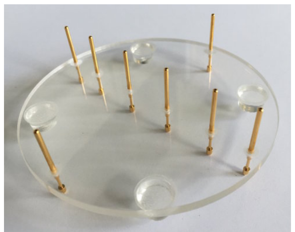
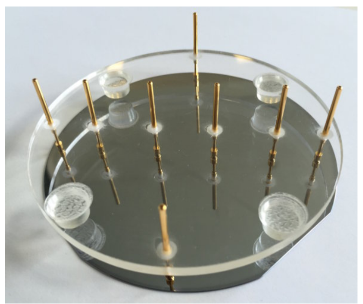
- Plexiglas plate with 8 spring-loaded pins
- An ohmic resistor
- Color stickers
Important precautions
- The silicon wafer provided can easily be broken if dropped or bent. Do not touch or scratch the shiny metallic surface.
Instructions
- In the experiment, the signal generator will be used as a DC voltage source. In this mode, the signal generator outputs a constant voltage between the voltage socket (5) and the GND socket (7). The numbers refer to the photograph shown in the general instructions.
- The voltage (range: - ) can be adjusted on the left potentiometer labeled adjust voltage (3) using the screwdriver.
- When performing this experiment, make sure that the loudspeaker drive section of the signal generator is turned off using the toggle switch (8). This can be checked by measuring the voltage between the speaker amplitude monitor socket (6) and the GND socket (7). If the loudspeaker drive section is off, the voltage between these two terminals is zero.
Part A. Four-point-probe (4PP) measurements (1,2 т.)
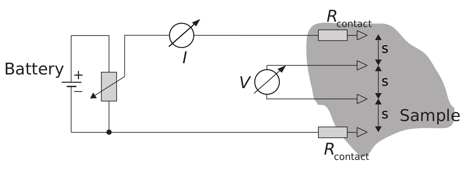
In order to measure the resistivity of a sample precisely, the contacts used for the voltage measurement and the contacts used for current injection should be separated.
This technique is called four-point-probe technique (4PP). The four contacts are arranged into a symmetric geometry that is as simple as possible: The current flows into the sample through one of the outer contacts (called source), then on all possible paths through the sample and out of the sample through the other contact (drain). In between, the voltage is measured over a certain path length on the sample.
Everything becomes quite simple if we have a symmetric setup, i.e. the same distance between all contacts and the contacts in the center of the sample as shown in following sketch:
The curve versus represents the -characteristics of the sample and allows the resistance of this sample segment to be determined. In the following we will only use the 4PP technique. To start, we will use the linear equidistant arrangement of four out of the eight probes (contacts) shown in the photograph.
For the following measurement, use the whole sheet of conducting paper.
Important hints for all following measurements:
- The long side of the sheet of paper is the reference side. The four probes should be aligned parallel to this side.
- Be careful to use the coated side (black), not the brown back side of the paper! You may mark the correct orientation with color stickers.
- Check that there are no holes or cuts in the paper.
- For these measurements, place the contacts as close to the center of the sample as possible.
- Press the contacts with enough force to ensure good contact for each of them. The plastic feet should just touch the surface.
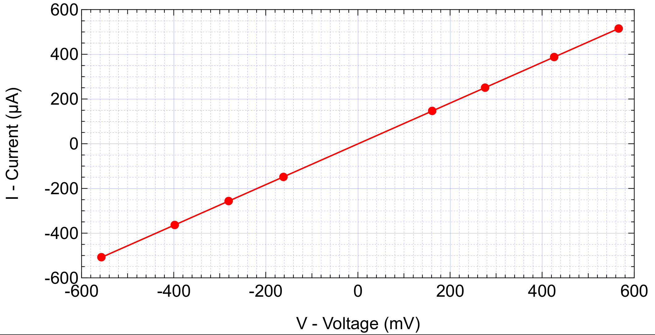
A.1 Four-point-probe (4PP) measurement: Measure the potential drop over a segment of length as function of current passing through this segment. Take in total at least 4 values, make a table and plot the voltage drop versus the current in Graph A.1. [0,6 т.]
A.2 Determine the effective electrical resistance that you obtained from Graph A.1. [0,2 т.]
A.3 Use Graph A.1 to determine the uncertainty on the resistance for the 4PP measurement. [0,4 т.]
Part B. Sheet resistivity (0,3 т.)
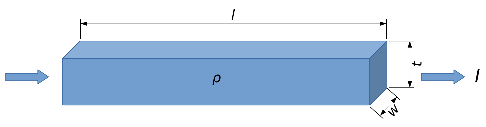
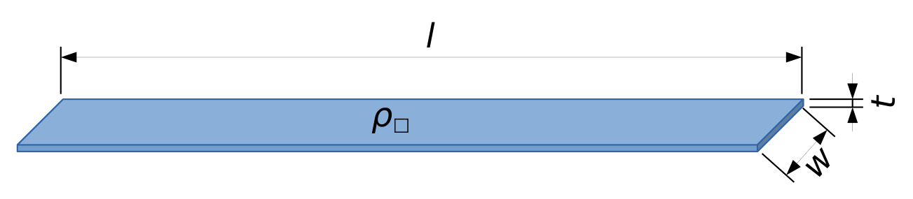
The resistivity represents a material property, by means of which the resistance of a 3D conductor of given dimensions and geometry is calculated. Here we consider a bar of dimensions length , width , and thickness :
The electrical resistance of the upper, thick conductor is given by:
On the same basis we may define the resistance of the 2D conductor of thickness and
using the sheet resistivity ("rho box"). Its unit is given in Ohms: .
Important: Eq. 2 is only valid for a homogeneous current density and constant potential in the cross-sectional plane of the conductor. In the case of point-like contacts on the surface this does not hold. Instead one can show that the sheet resistivity is related to the resistance in that case by
for .
B.1 Calculate the sheet resistivity of the paper from the 4PP measurement in part A. We will call this particular value (and the measured resistance from part A ) because the sample dimensions of the whole sheet are much larger than the spacing of the contacts : . [0,3 т.]
Part C. Measurements for different sample dimensions (3,2 т.)
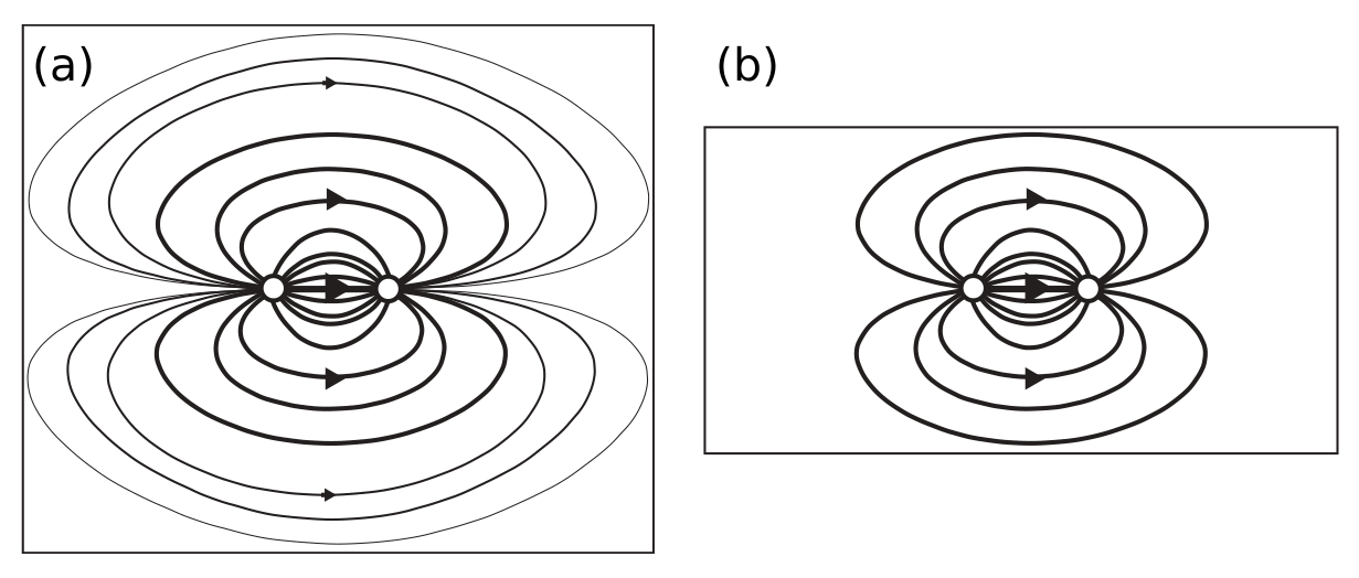
Up to now, the finite sample dimensions and were not taken into account. If the sample becomes smaller, it can carry less current if the voltage is kept constant: If we apply a voltage between the two point contacts (white circles), current will flow on all possible, non-crossing paths through the sample as visualized by the lines: the longer the line, the smaller the current as indicated by the line thickness. For a small sample (b) and the same applied voltage, the total current decreases because there are less possible pathways. Thus, the measured resistance will increase:
The (sheet) resistivity will not change as function of sample size. Thus, in order to convert the measured resistance into a resistivity using Eq. 3, we need to introduce a correction factor :
For a sample of length the factor only depends on the ratio and is larger than : . For the sake of simplicity we will focus on the dependence on the width and only ensure that the sample is long enough for our measurements. We assume that the value approaches the correct result for large dimensions:
C.1 Using the 4PP-method, measure the resistance for 4 values within the range 0.3 to 5.0 and record your results in Table C.1. Ensure that the sample length is larger than five times the probe spacing: and that the length of the samples is always taken along the same (long) side of the sheet of paper. For each value of measure the voltage for 4 different current values and calculate the average resistance out of the 4 measurements. Enter your results in Table C.1. [3 т.]
C.2 Compute for each of these measurements. [0,2 т.]
Part D. Geometrical correction factor: scaling law (1,9 т.)
You have seen in part C that the measured resistivity scales with the ratio of width to probe distance . Starting from the data acquired in part C we choose the following generic function to describe the data in the range of the measurements:
Note that for very large , must be .
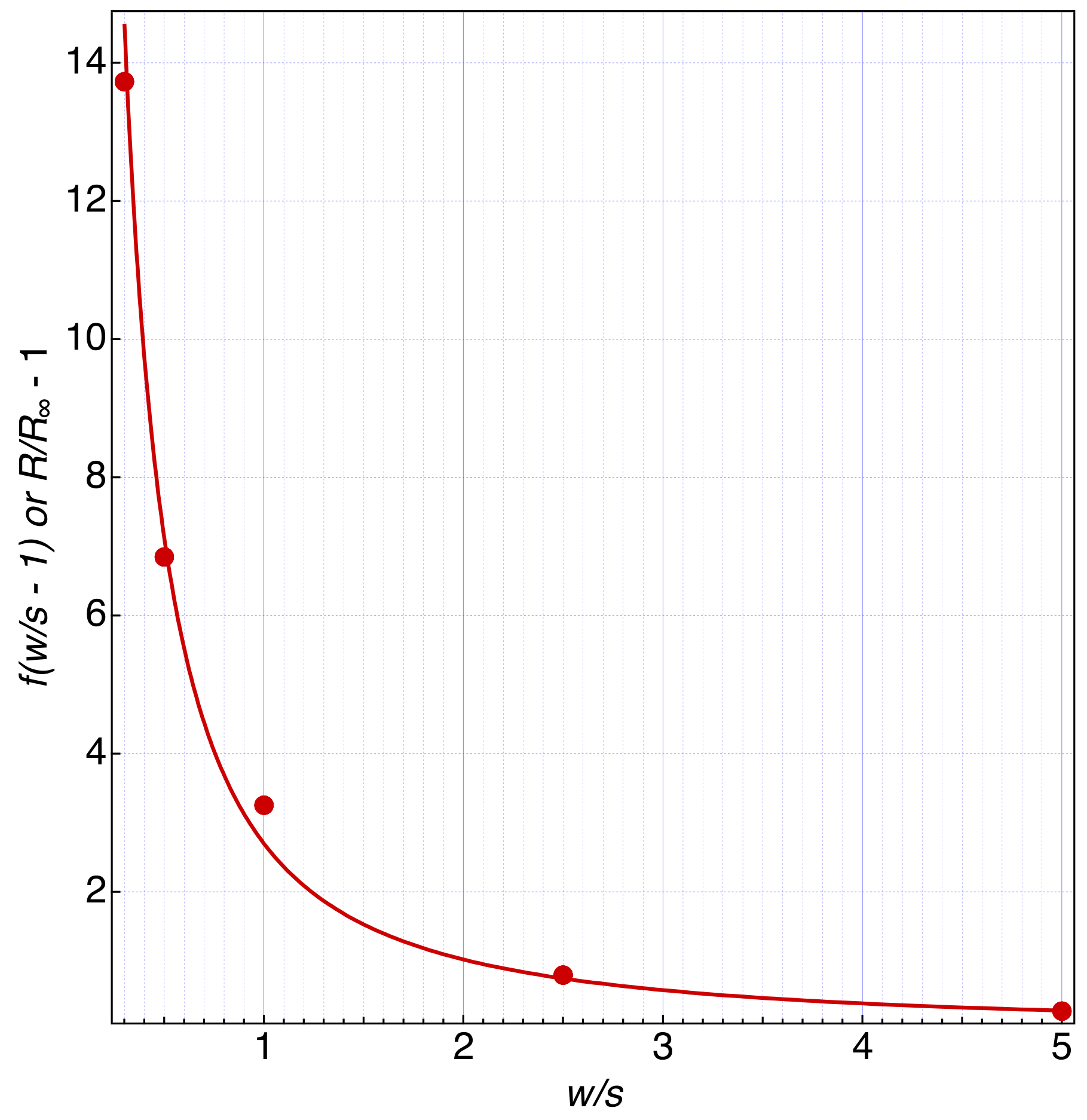
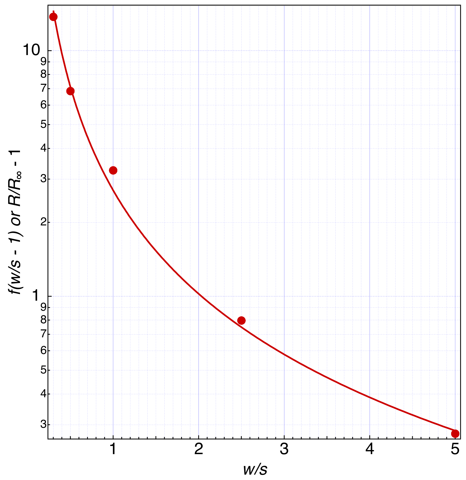
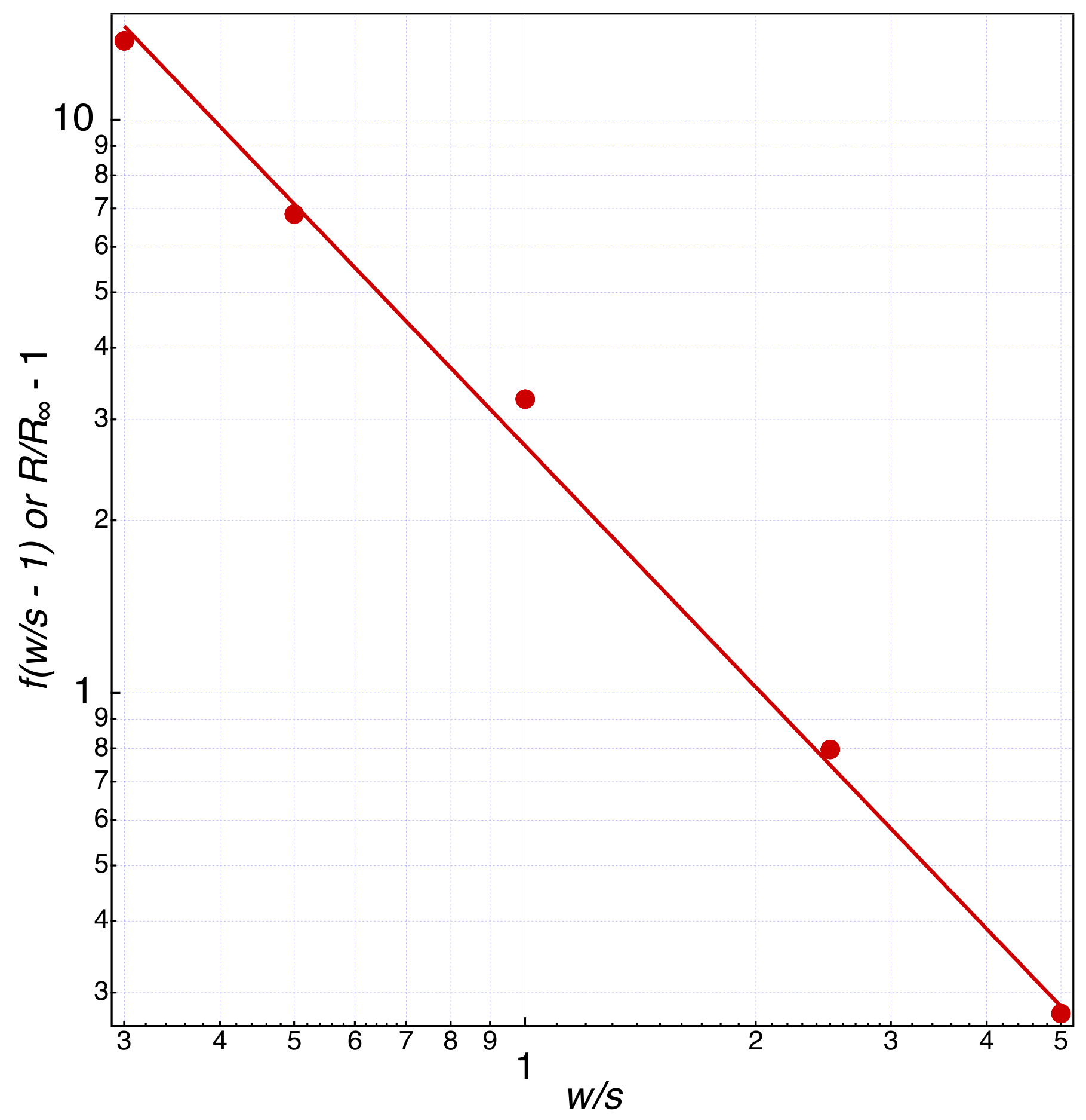
D.1 In order to fit a model curve using Eq. 6 and the data , taken in part C, choose the most appropriate graph paper (linear Graph D.1a, semi-logarithmic Graph D.1b, or double-logarithmic Graph D1.c) to plot the data. [1 т.]
D.2 Deduce the parameters and from your fit. [0,9 т.]
Part E. The silicon wafer and the van der Pauw-method (3,4 т.)
In the semi-conductor industry, knowledge of the electrical (sheet) resistance of semi-conductors and thin metal layers is very important because it determines the properties of devices. In the following you will work with the silicon wafer. The semi-conducting wafer is coated with a very thin layer of chromium metal (on the shiny side).
Open the wafer container (rotate in the sense of the arrow RELEASE) and take the wafer out. Be careful not to drop or to break it nor to scratch or touch the shiny surface. For the measurements place it on the table with the shiny side point up towards you.
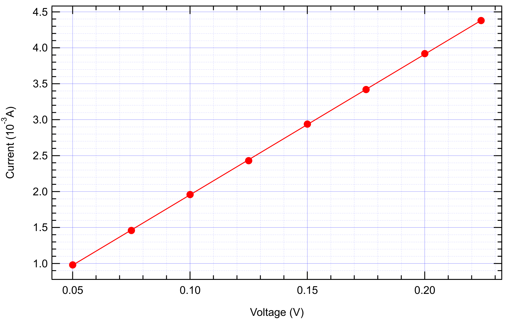
E.1 Use the same 4PP setup as previously to measure the voltage as function of current .
Write down the reference number of your wafer in the Answer Sheet. You find this number on the plastic wafer holder. [0,4 т.]
E.2 Plot the data in Graph E.2 and determine the resistance . [0,4 т.]
E.3 In order to determine the correction for a circular sample like the wafer, we will approximate the effective width of the sample by the diameter of the wafer. Under this assumption calculate the ratio . Use the fit function in Eqn. 6 and your parameters and to determine the correction factor for the wafer measurement. [0,2 т.]
E.4 Calculate the sheet resistivity of the chromium layer using Eq. 4. [0,1 т.]
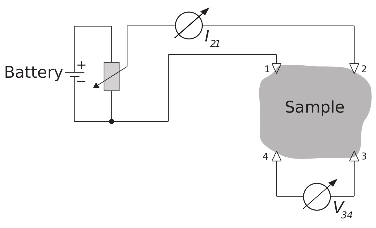
In order to measure the sheet resistivity precisely without need for geometrical corrections, Philips engineer L.J. van der Pauw developed a simple measurement scheme: The four probes are mounted at the circumference of a sample of arbitrary shape as shown in the figure (numbered 1 through 4). The current flows through two adjacent probes, e.g. probes 1 and 2, and the voltage is measured between probes 3 and 4. This yields a resistance value .
For symmetry reasons and . Van der Pauw showed that for an arbitrary but simply connected shape (no holes) of the sample and point-like contacts the following equation holds:
Connect the four spring contacts such that the measurement probes form a square. Connect two adjacent contacts to the current source with the amperemeter, and connect the two remaining spring contacts with the voltmeter. Rotate the square until one of its edges is parallel to the flat of the wafer.
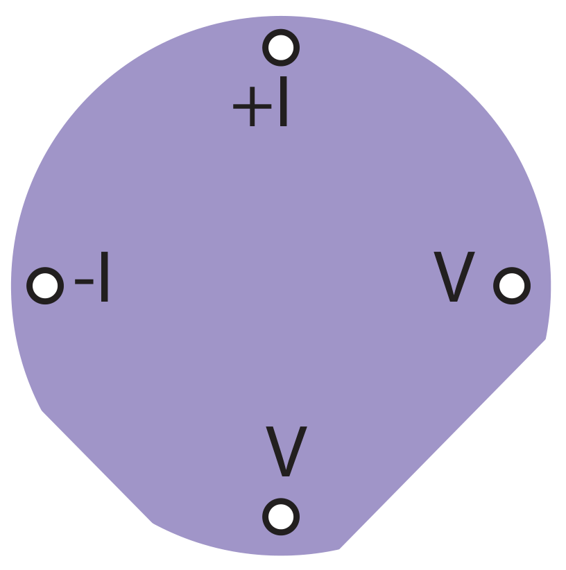
E.5 Sketch the orientation of the current carrying contacts and the orientation of the flat of the wafer. Measure the voltage for at least in total 6 different values of current , roughly equally spaced. Enter the results into Table E.5. [0,6 т.]
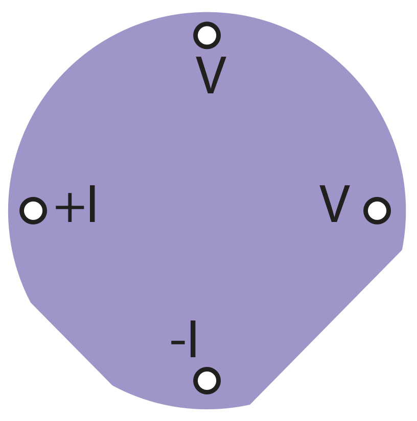
E.6 Repeat the procedure arranging the current carrying contacts perpendicular to those used in the first step. Enter the results into Table E.6. [0,6 т.]
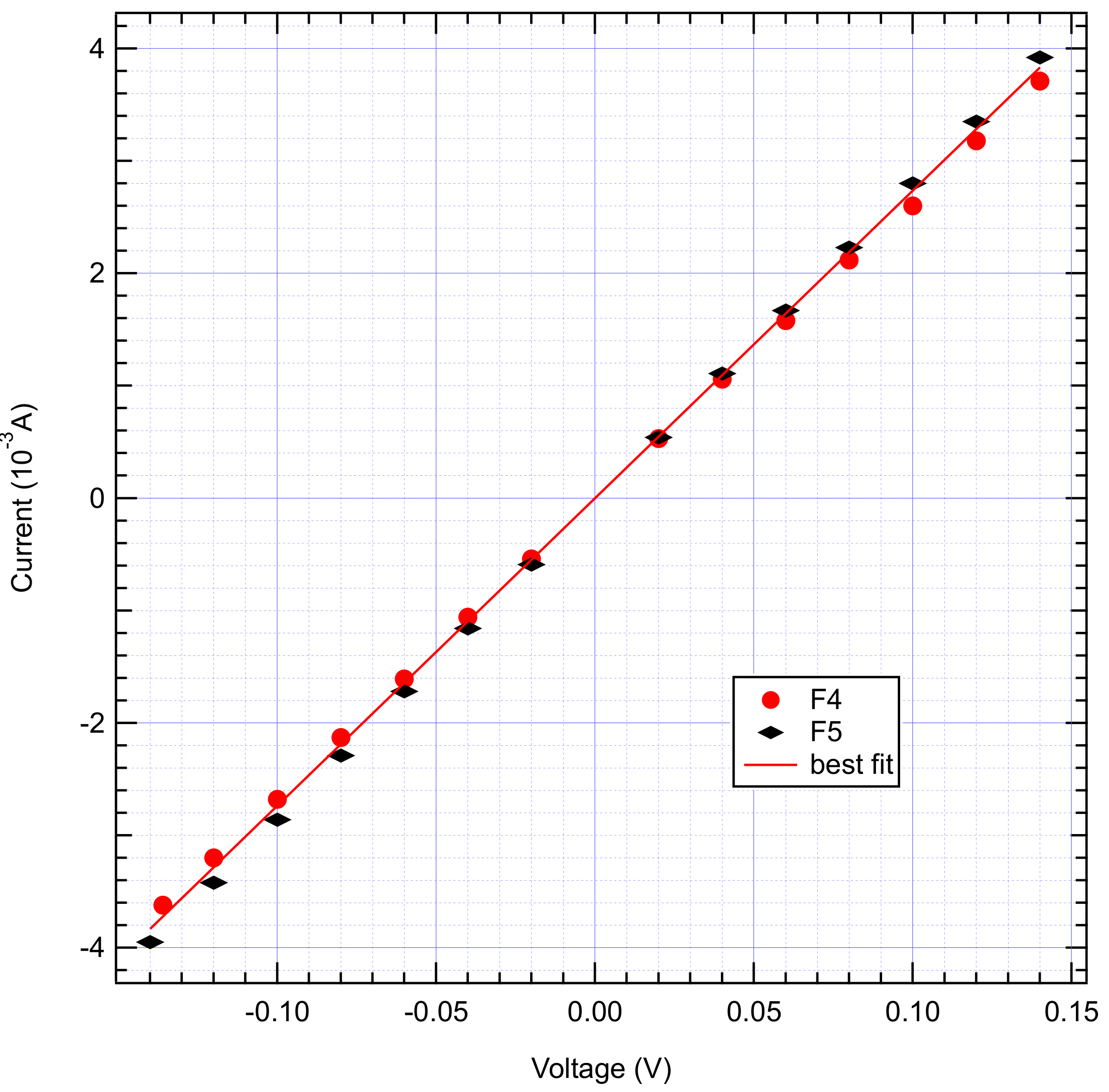
E.7 Plot all the data together in a single graph Graph E.7 using different colors and/or symbols. Determine the mean value from the two curves. [0,5 т.]
E.8 Replacing all resistances by , solve Eqn. 7 for and calculate the sheet resistivity of the chromium layer. [0,4 т.]
E.9 Compare the result of the measurement taken with the linear arrangement (E.4) and the result of the van der Pauw method (E.8). Give the difference of the two measurements as relative error in percent. [0,1 т.]
E.10 The chromium (Cr) layers have a nominal thickness of . Use this value and the final results of the van der Pauw method to calculate the resistivity of Cr using Eqns. 1 and 2. [0,1 т.]
Отговори
Part A. Four-point-probe (4PP) measurements, A.2 1.08 kΩ
Sample result from the official answer sheet; the value depends on the individual measurement.
Part A. Four-point-probe (4PP) measurements, A.3 ΔR = ±1 Ω
Sample result from the official answer sheet.
Part B. Sheet resistivity, B.1 4.89 kΩ
Sample result from the official answer sheet (printed as ρ□ ≡ ρ∞ = 4.89 kΩ).
Part D. Geometrical correction factor: scaling law, D.1 double-logarithmic graph paper (Graph D1c)
Official answer sheet: linear and semi-log scales are marked wrong; on the double-log scale the parameters can be deduced by fitting a line.
Part D. Geometrical correction factor: scaling law, D.2 a = 2.7, b = −1.4
Sample result from the official answer sheet.
Part E. The silicon wafer and the van der Pauw-method, E.2 51.1 Ω
Sample result from the official answer sheet.
Part E. The silicon wafer and the van der Pauw-method, E.3 1.284
Official answer sheet: w = 10 cm → w/s = 5, f(w/s) = 1.284 (sample result).
Part E. The silicon wafer and the van der Pauw-method, E.4 180 Ω
Sample result from the official answer sheet.
Part E. The silicon wafer and the van der Pauw-method, E.7 36.5 Ω
Sample result from the official answer sheet.
Part E. The silicon wafer and the van der Pauw-method, E.8 ≈ Ω
Sample result from the official answer sheet.
Part E. The silicon wafer and the van der Pauw-method, E.9 9.1 %
Sample result from the official answer sheet (0.091).
Part E. The silicon wafer and the van der Pauw-method, E.10 0.00000132 Ω·m
Sample result from the official answer sheet.
Решение
Problem 1 : Electrical conductivity in two dimensions - Answer Sheet (10 points)
Part A. Four-point-probe (4PP) measurements (1.2 points)
A1 (0.6 pts)
| (A) | (mV) | (A) | (mV) |
|---|---|---|---|
| 251 | 276 | -148 | -162 |
| 516 | 566 | -256 | -281 |
| 388 | 426 | -363 | -398 |
| 147 | 161 | -507 | -557 |
Plot your data in the graph B1
A2 (0.2 pts)
A3 (0.4 pts)
Part B. Sheet resistivity (0.3 points)
B1 (0.3 pts)
Part C. Measurements for different sample dimensions (3.2 points)
C1 (3 pts) and C2 (0.2 pts)
| I (A) | V (mV) | R() (k) | R (k) | |||
|---|---|---|---|---|---|---|
| 0.3 | 92 | 1477 | 16.1 | 15.9 | 14.7 | |
| 0.3 | 74 | 1184 | 16 | |||
| 0.3 | 57 | 914 | 16 | |||
| 0.3 | 41 | 651 | 15.9 | |||
| 0.3 | 23 | 358 | 15.6 | |||
| 0.5 | 154 | 1306 | 8.5 | 8.5 | 7.8 | |
| 0.5 | 127 | 1079 | 8.5 | |||
| 0.5 | 97 | 824 | 8.5 | |||
| 0.5 | 67 | 567 | 8.5 | |||
| 0.5 | 38 | 321 | 8.4 | |||
| 1 | 233 | 1071 | 4.6 | 4.6 | 4.3 | |
| 1 | 174 | 799 | 4.6 | |||
| 1 | 135 | 621 | 4.6 | |||
| 1 | 101 | 465 | 4.6 | |||
| 1 | 59 | 271 | 4.6 | |||
| 2.5 | 389 | 749 | 1.9 | 1.9 | 1.8 | |
| 2.5 | 319 | 635 | 2 | |||
| 2.5 | 237 | 457 | 1.9 | |||
| 2.5 | 151 | 291 | 1.9 | |||
| 2.5 | 74 | 143 | 1.9 | |||
| 5 | 467 | 648 | 1.4 | 1.4 | 1.3 | |
| 5 | 419 | 577 | 1.4 | |||
| 5 | 363 | 499 | 1.4 | |||
| 5 | 289 | 398 | 1.4 | |||
| 5 | 185 | 254 | 1.4 |
Part D. Geometrical correction factor (1.9 points)
D1 (1.0 pts)
Plot your data on the appropriate graph paper: linear (Graph E1a), semi-logarithmic (D1b) or double-logarithmic (D1c) on the following pages.
D2 (0.9 pts)
Graph D1a: linear scale: vs
Wrong. The usage of linear scale does not allow for deduction of the parameters.
Graph D1b: semi-log scale: vs
Wrong. The usage of semi-log scale does not allow for deduction of the parameters.
Graph D1c: double-log scale: vs
Correct. The parameters can be deduced by fitting a line.
Part E. van der Pauw-method (3.4 points)
Note the number of your wafer here: 99 (between 1 - 450)
E1 (0.4 pts)
| (mA) | (mV) | (mA) | (mV) |
|---|---|---|---|
| 0.98 | 50 | 2.94 | 150 |
| 1.46 | 75 | 3.42 | 175 |
| 1.96 | 100 | 3.92 | 200 |
| 2.43 | 125 | 4.38 | 224 |
E2 (0.4 pts)
E3 (0.2 pts)
E4 (0.1 pts)
E5 (0.6 pts)
Sketch (orientation of the current):
| mV | mA |
|---|---|
| 140 | 3.71 |
| 120 | 3.18 |
| 100 | 2.66 |
| 80 | 2.12 |
| 60 | 1.58 |
| 40 | 1.06 |
| 20 | 0.53 |
| -20 | -0.54 |
| -40 | -1.06 |
| -60 | -1.61 |
| -80 | -2.13 |
| -100 | -2.68 |
| -120 | -3.2 |
| -136 | -3.62 |
E6 (0.6 pts)
Sketch (orientation of the current):
| 140 | 3.92 |
| 120 | 3.35 |
| 100 | 2.8 |
| 80 | 2.23 |
| 60 | 1.67 |
| 40 | 1.11 |
| 20 | 0.54 |
| -20 | -0.59 |
| -40 | -1.16 |
| -60 | -1.72 |
| -80 | -2.29 |
| -100 | -2.86 |
| -120 | -3.42 |
| -140 | -3.95 |
E7 (0.5 pts)
E8 (0.4 pts) Calculation:
E9 (0.1 pts)
E10 (0.1 pts)
Resistivity of the Cr thin film
Оригинал в Архива: exp1.pdf · официални решения: exp1_sol.pdf