IPhO 2016, Експеримент — Задача 2. Jumping beads - A model for phase transitions and instabilities
IPhO 2016 International Physics Olympiad Switzerland Liechtenstein — Experiment, English (Official), Q2 · 10 т.
Условие
Please read the general instructions in the separate envelope before you start this problem.
Introduction
Phase transitions are well known from every day life, e.g. water takes different states like solid, liquid and gaseous. These different states are separated by phase transitions, where the collective behaviour of the molecules in the material changes. Such a phase transition is always associated with a transition temperature, where the state changes, i.e. the freezing and boiling temperatures of water in the above examples.
Phase transitions are however even more wide-spread and also occur in other systems, such as magnets or superconductors, where below a transition temperature the macroscopic state changes from a paramagnet to a ferromagnet and a normal conductor to a superconductor, respectively.
All of these transitions can be described in a common framework when introducing a so-called order-parameter. For instance, in magnetism the order parameter is associated with the alignment of the magnetic moments of the atoms with a macroscopic magnetisation.
In the so-called continuous phase transitions, the order parameter will always be zero above the critical temperature and then grow continuously below it, as shown in the schematic for a magnet in figure 1 below. The transition temperature of a continuous phase transition is called the critical temperature. The figure also contains a schematic representation of the microscopic order or disorder in the case of a magnet, where the individual magnetic moments align in the ferromagnetic state to give rise to a macroscopic magnetization, whereas they are randomly oriented in the paramagnetic phase yielding a macroscopic magnetization of zero.
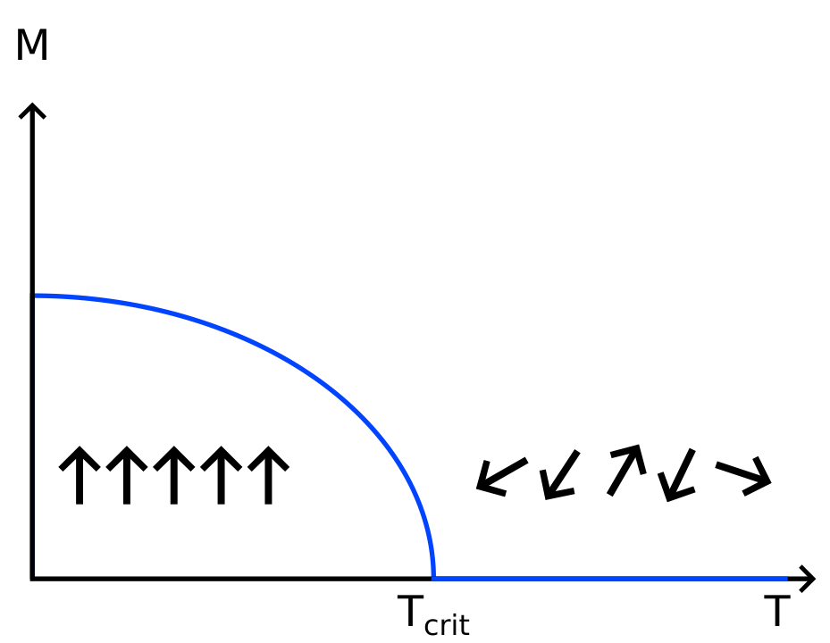
For continuous phase transitions, one generally finds that the order parameter close to a transition follows a power-law, e.g. in magnetism the magnetization below the critical temperature, , is given by:
where is temperature. What is even more stunning is that this behaviour is universal: the exponent of this power-law is the same for many different kinds of phase transition.
Task
We will study a simple example where some of the features of continuous phase transitions can be investigated, such as how an instability leads to the collective behaviour of the particles and thus to the phase transition as well as how the macroscopic change depends on an excitation of the particles.
In common phase transitions this excitation is usually driven by temperature. In our example, the excitation consists of the kinetic energy of the particles accelerated by the loudspeaker. The macroscopic change corresponding to the phase transition that we study here consists of the sorting of beads into one half of a cylinder, which is separated by a small wall.
Increasing the amplitude from where particles have sorted into one half of the cylinder, you will find that eventually the particles distribute equally between the two halves. This corresponds to having heated past the critical temperature.
Your objective is to determine the critical exponent for the model phase transition studied here.
List of material
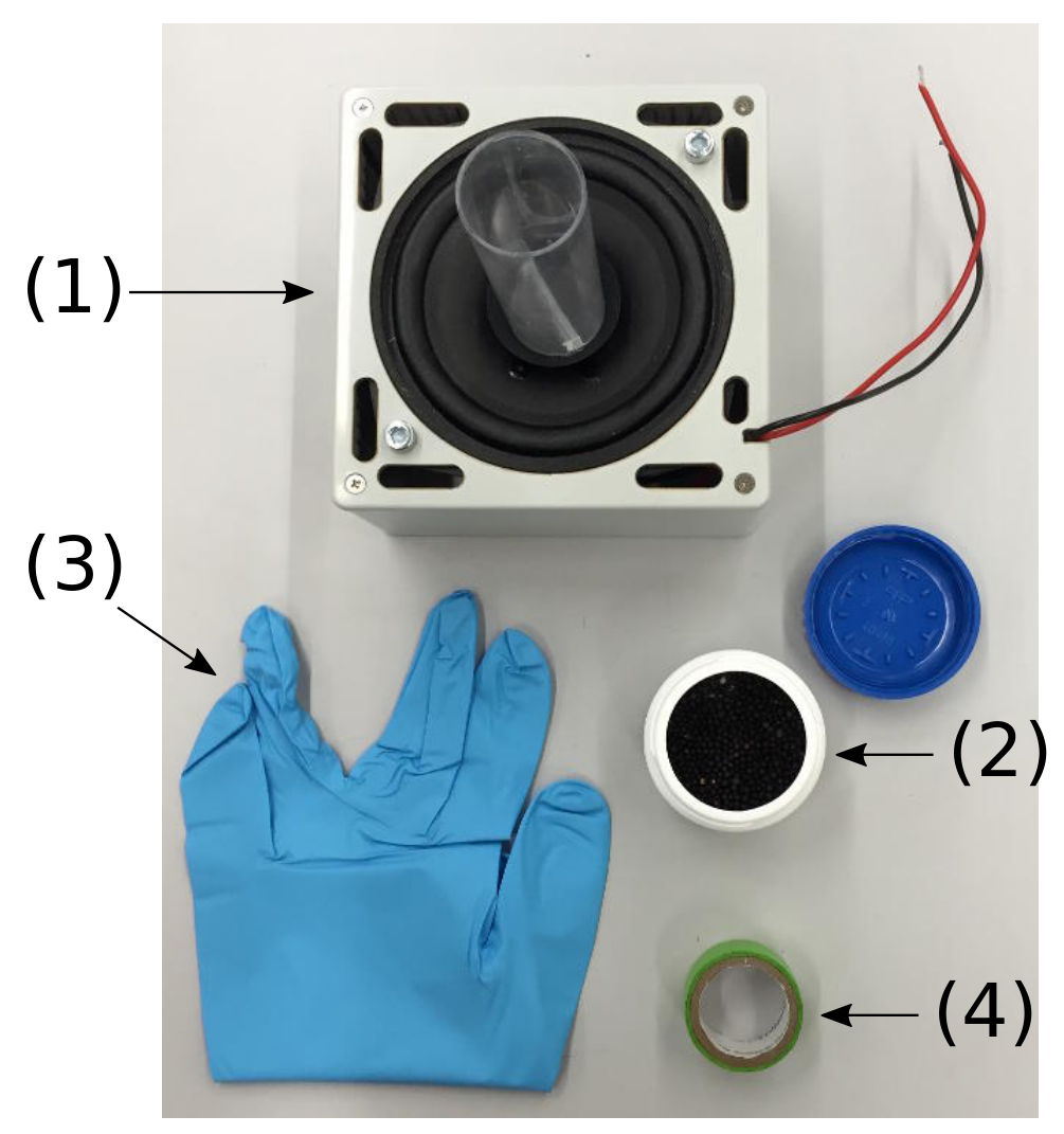
- Loudspeaker assembly with plastic cylinder mounted on top
- About 100 poppy seeds (in a plastic container)
- A glove
- Sticky tape
Important precautions
- Do not apply an excessive lateral force to the plastic cylinder mounted on the loudspeaker. Note that no replacements will be provided in case of torn loudspeaker membranes or torn off plastic cylinder.
- Turn off the loudspeaker assembly whenever not in use, in order to avoid unnecessary drain of the battery.
- In this experiment, a saw-tooth signal is output on the loudspeaker terminals located at the side of the signal generator.
- The amplitude of the saw-tooth signal can be adjusted using the right potentiometer labeled speaker amplitude (4). A DC voltage proportional to the signal amplitude is output on the speaker amplitude monitor socket (6) (with respect to the GND socket (7)). The numbers refer to the photograph (Figure 2) shown in the general instructions.
- The speaker membrane is delicate. Make sure that you do not apply unnecessary pressure on it by any means either vertically or laterally.
Part A. Critical excitation amplitude (3.3 points)
Before you start the actual tasks of this problem, wire up the loudspeaker to the terminals on the side of the signal generator (make sure you use the correct polarity). Put some (e.g. ) poppy seeds into the cylinder mounted on the loudspeaker and use a piece cut from the glove provided to close the cylinder at the top in order to keep the poppy seeds in the cylinder. Switch on the excitation using the toggle switch and adjust the amplitude by turning the right potentiometer labeled speaker amplitude (4) by means of the screwdriver provided. Observe the sorting of the beads by testing different amplitudes.
The first task is to determine the critical excitation amplitude of this transition. In order to do this, you have to determine the number of beads and in the two compartments (choosing the compartment labels such that ) as a function of the displayed amplitude , which is the voltage measured at the speaker amplitude socket (6). This voltage is proportional to the amplitude of the saw-tooth waveform driving the loudspeaker. Make at least 5 measurements per voltage.
Hint:
- In order to always have a motion in the particles you study, only investigate amplitudes corresponding to speaker amplitude voltages exceeding . Start with watching the behaviour of the system just by varying the voltage slowly without any counting of he beads. It can be that some of the beads stick to the ground due to electrostatic reasons. Don't count these beads.
A.1 Record your measurements of the number of particles and in each half of the container for various amplitudes in Table A.1. [1,2 т.]
A.2 Calculate the standard deviation of your measurements of and and list your results in Table A.1. Plot and as a function of the displayed amplitude in Graph A.2, including their uncertainties. [1,1 т.]
A.3 Based on your graph, determine the critical displayed amplitude at which , after waiting until a stationary state is reached. [1 т.]
Part B. Calibration (3.2 points)
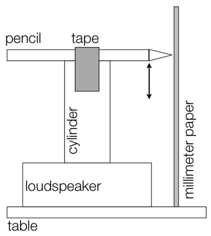
The displayed amplitude , corresponds to a voltage applied to the loudspeaker. However, the physically interesting quantity is the maximum displacement of the oscillation of the loudspeaker, since this relates to how strongly the beads are excited. Therefore, you need to calibrate the displayed amplitude. For this purpose, you can use any of the provided material and tools.
B.1 Sketch the setup you use to measure the excitation amplitude, i.e. the maximum travel distance (in ) of the loudspeaker in one period of oscillation. [0,5 т.]
B.2 Determine the amplitude in for a suitable number of points, i.e. record the amplitude as a function of displayed amplitude in Table B.2 and indicate the uncertainties of your measurements. [0,8 т.]
B.3 Plot your data in Graph B.3, including the uncertainties. [1 т.]
B.4 Determine the parameters of the resulting curve, using an appropriate fit to determine the calibration function . [0,8 т.]
B.5 Determine the critical excitation amplitude of the poppy seeds. [0,1 т.]
Part C. Critical exponent (3.5 points)
In our system, the temperature corresponds to the input kinetic energy of the excitation. This energy is proportional to the speed squared of the loudspeaker, i.e. to , where is the frequency of the oscillation. We will now test this dependence and determine the exponent of the power-law governing the behavior of the order parameter (see Eq. 1).
C.1 The imbalance is a good candidate for an order parameter for our system in that it is zero above the critical amplitude and equal to at low excitation. Determine this order parameter as a function of the amplitude . Record your results in the Table C.1. [1,1 т.]
C.2 Plot the imbalance as a function of , in Graph C.2, where both axes have logarithmic scales (double-logarithmic plot). You can use the Table C.1 for your calculations. The points on the plot may seem not to obey a linear relation, but a linear regression should be made nevertheless, to match the critical exponent formula. [1 т.]
C.3 Determine the exponent and estimate the error. [1,4 т.]
Отговори
A.3 1.25 V
Official sample result: ; experimental values depend on the apparatus.
B.4
Official sample fit; experimental values depend on the apparatus.
B.5 4.4 mm
Official sample result: .
C.3 0.6
Official result: critical exponent .
Решение
Problem 2 : Solution – Jumping Beads - a model for phase transitions and instabilities (10 points)
Part A. Critical driving amplitude (3.3 points)
A1 (1.2 pts)
Total number of seeds: .
Number of readings: .
| , [V] | ||||||||||
|---|---|---|---|---|---|---|---|---|---|---|
| 1.00 | 1 | 5 | 2 | 1 | 2 | 2 | 2.2 | 47.8 | 1.5 | 0.6 |
| 1.05 | 1 | 0 | 2 | 3 | 1 | 2 | 1.5 | 48.5 | 1.1 | 0.5 |
| 1.10 | 4 | 4 | 1 | 7 | 3 | 5 | 4.0 | 46.0 | 2.0 | 0.8 |
| 1.15 | 26 | 5 | 18 | 7 | 18 | 7 | 13.5 | 36.5 | 8.4 | 3.4 |
| 1.20 | 13 | 16 | 27 | 12 | 17 | 13 | 16.4 | 33.7 | 5.6 | 2.3 |
| 1.25 | 26 | 28 | 22 | 22 | 14 | 23 | 22.5 | 27.5 | 4.8 | 2.0 |
| 1.30 | 27 | 24 | 8 | 22 | 22 | 21 | 20.7 | 29.3 | 6.6 | 2.7 |
| 1.40 | 22 | 18 | 17 | 23 | 23 | 25 | 21.4 | 28.7 | 3.2 | 1.3 |
| 1.50 | 19 | 27 | 27 | 24 | 19 | 21 | 22.8 | 27.2 | 3.7 | 1.5 |
| 1.60 | 27 | 15 | 23 | 23 | 23 | 30 | 23.5 | 26.5 | 5.1 | 2.1 |
Plot the data in the graph A2.
A2 (1.1 pts)
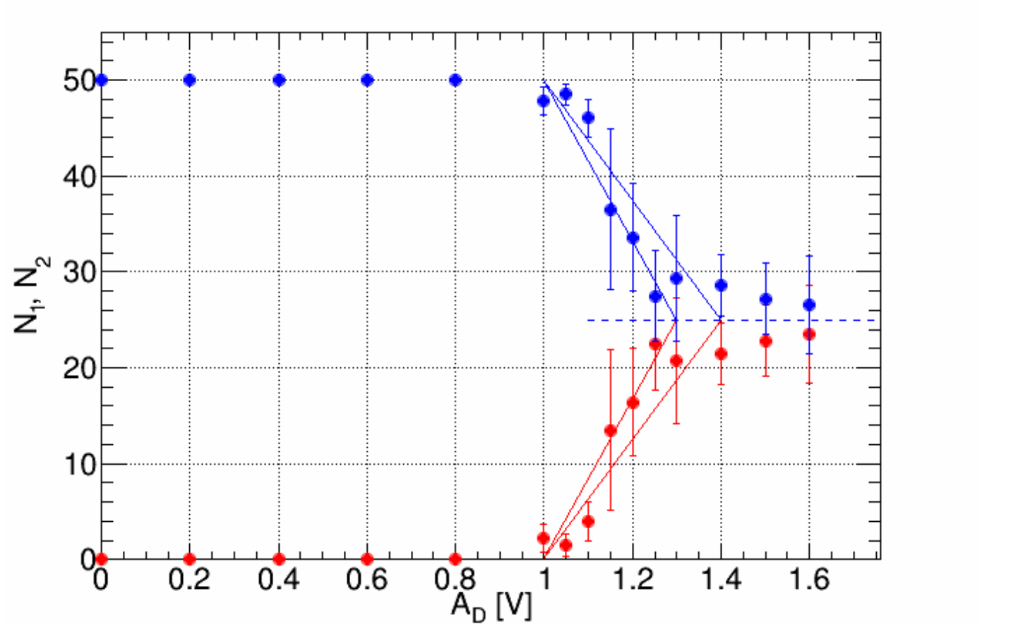
Error bars represent either standard deviation () or standard error (SE).
A3 (1.0 pts)
Part B. Calibration (3.2 points)
B1 (0.5 pts)
B2 (0.8 pts)
| [V] | 0.3 | 0.4 | 0.5 | 0.6 | 0.7 | 0.8 | 0.9 | 1.0 | 1.1 | 1.2 | 1.3 | 1.4 | 1.5 | 1.6 | 1.7 | 1.8 | 1.9 | 2.0 | 2.1 |
|---|---|---|---|---|---|---|---|---|---|---|---|---|---|---|---|---|---|---|---|
| [mm] | 1.0 | 1.5 | 2.0 | 2.2 | 2.6 | 3.0 | 3.2 | 3.4 | 4.0 | 4.1 | 4.2 | 4.5 | 4.8 | 5.0 | 5.0 | 5.1 | 5.1 | 5.2 | 5.2 |
Instrumental error mm.
B3 (1.0 pts)
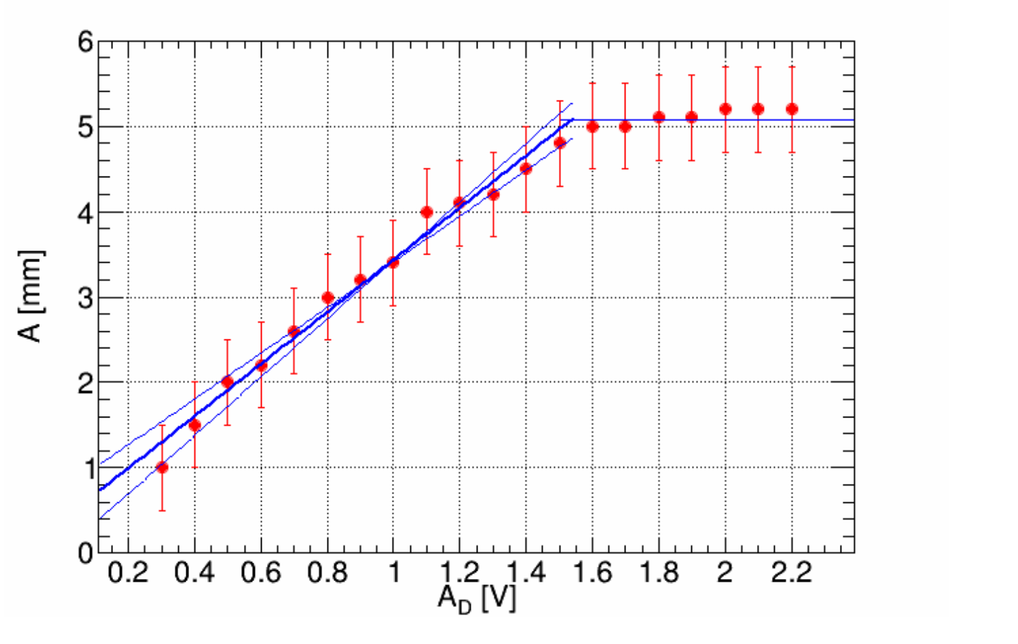
B4 (0.8 pts)
,
where:
,
B5 (0.1 pts)
Part C. Critical exponent (3.5 points)
C1 (1.1 pts)
| , [V] | , [mm] | ||
|---|---|---|---|
| 1.00 | 3.5 | 0.91 | 6.8 |
| 1.05 | 3.6 | 0.94 | 5.7 |
| 1.10 | 3.8 | 0.84 | 4.6 |
| 1.15 | 3.9 | 0.46 | 3.5 |
| 1.20 | 4.1 | 0.35 | 2.2 |
| 1.25 | 4.2 | 0.10 | 1.0 |
| 1.30 | 4.4 | 0.17 | 0.3 |
| 1.40 | 4.7 | 0.15 | |
| 1.50 | 5.0 | 0.09 | |
| 1.60 | 5.3 | 0.06 |
Plot the data in the graph C2.
C2 (1.0 pts)
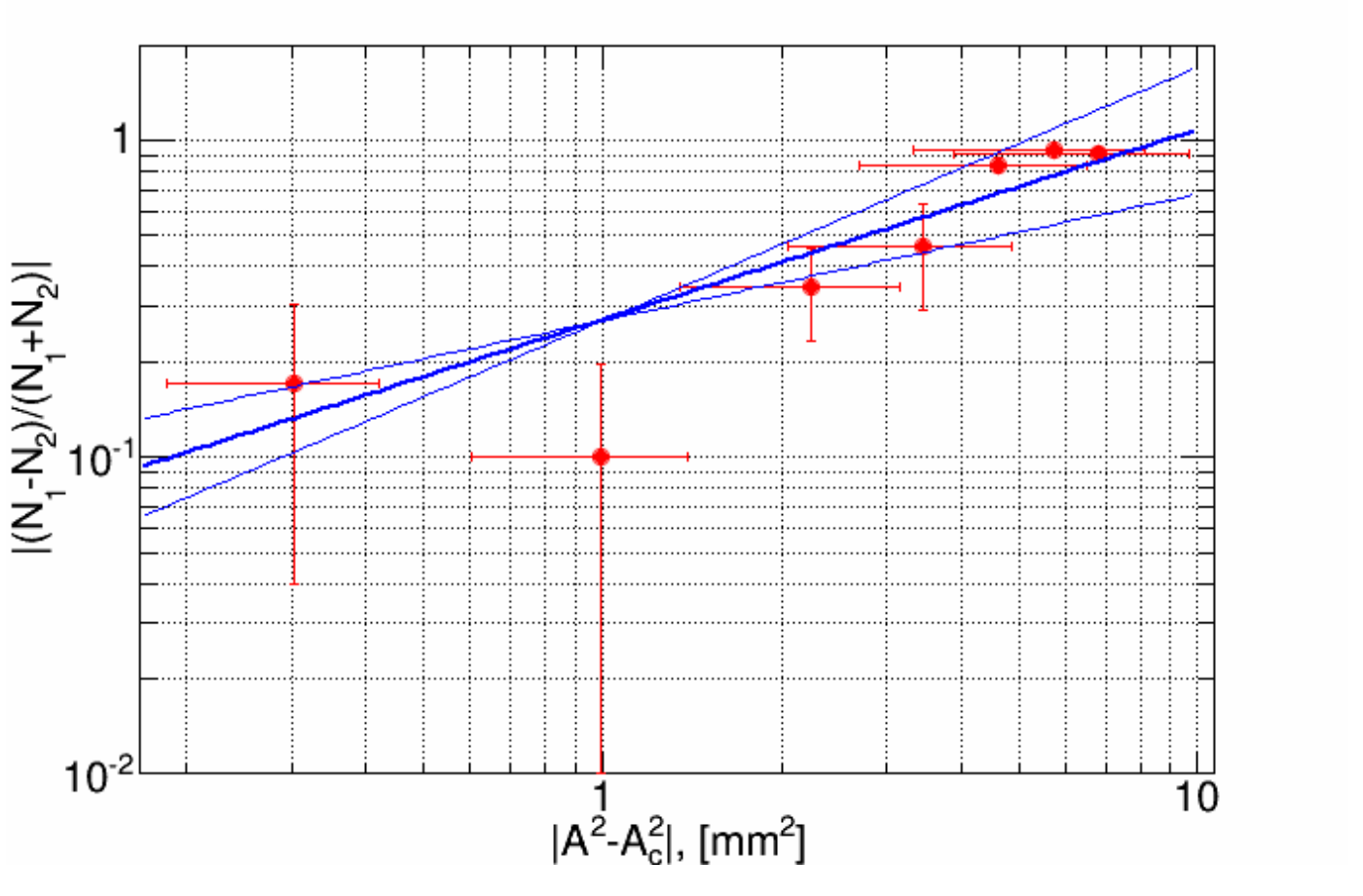
C3 (1.4 pts)
, where , .
Critical exponent .
Оригинал в Архива: exp2.pdf · официални решения: exp2_sol.pdf