Съдържание
УсловиеI. IntroductionII. ObjectivesIII. List of MaterialsIV. Experiments and TasksA: Measurement of Refractive Index Gradient of Salt Water Solution (4.5 points)B: Determination of Diffusion Coefficient (4.2 points)C. Nonlinear diffusion (1.3 points)AE1 — Determination of Refractive Index Gradient and Diffusion Coefficient of Salt Solution from Laser Deflection Measurement (10 pt.)ОтговориРешениеIPhO 2017, Експеримент — Задача 1. Determination of Refractive Index Gradient and Diffusion Coefficient of Salt Solution from Laser Deflection Measurement
Determination of Refractive Index Gradient and Diffusion Coefficient of Salt Solution from Laser Deflection Measurement · 18 юли 2017 г. · 10 т.
Внимание: Бележка към темата
Several official marking columns are vertically displaced from their answer columns. Their entries are preserved in each column’s printed order; no new row correspondence is imposed. The official key’s printed data-count labels and all sample rows are retained.
General instructions: Experimental Examination
July 18, 2017
The experimental examination lasts for 5 hours and is worth a total of 20 points.
Before the exam
- You must not open the envelopes containing the problems before the sound signal indicating the beginning of the examination.
- The beginning and end of the examination will be indicated by a sound signal. There will be announcements every hour indicating the elapsed time, as well as fifteen minutes before the end of the examination (before the final sound signal).
During the exam
- Dedicated answer sheets are provided for writing your answers. Enter the observations into the appropriate tables, boxes or graphs in the corresponding answer sheet. For every problem, there are work sheets for carrying out detailed work. Be sure to always use the work sheets that belong to the problem you are currently working on (check the problem number in the header). If you have written something on any sheet which you do not want to be graded, cross it out. Only use the front side of every page. Do not forget to put your student code numbers in each working sheets or answer sheets in the field provided. Answers or working results will not be graded if there is no student code numbers written.
- In your answers, try to be as concise as possible: use equations, logical operators and sketches to illustrate your thoughts whenever possible. Avoid the use of long sentences.
- Explicit error calculation is not required unless explicitly asked for. However, you are asked to give an appropriate number of significant digits when stating numbers. Also, you should decide on the appropriate number of data points or measurement repetitions unless specific instructions are given.
- You may often be able to solve later parts of a problem without having solved the previous ones.
- You are not allowed to leave your working place without permission. If you need any assistance (need to refill your drinking water bottle, broken calculator, need to visit a restroom, etc.), please draw the attention of a supervisor by lifting one of the three flags into the air ("Refill my water bottle, please", "I need to go to the toilet, please", or "I need help, please" in all other cases).
At the end of the exam
- At the end of the examination you must stop writing immediately.
- For every problem, sort the corresponding sheets in the following order: questions, answer sheets, work sheets.
At the end of the exam — continued
- For E1 (Experimental Problem No. 1) you need to enclose the millimeter block paper that has been used for making the deflactogram. Please make sure that you have written your student code numbers and the concentration of the solutions that you used on this millimeter block paper.
- You must write the number and total number of pages used on your working sheets at the bottom of each pages.
- Put all the sheets belonging to one problem into the same envelope. Also put the general instructions into the remaining separate envelope (if available or just put it in outside the envelope if remaining separate envelope is not available). Also hand in empty sheets. You are not allowed to take any sheets of paper out of the examination area.
- Leave your writing equipment (provided by the committee, if any) as well as the provided calculator on the experiment table.
- Wait at your table until your envelopes and all the necessary equipment are collected. Once all envelopes and equipment are collected, your guide will escort you out of the examination area. Don’t forget to take your water bottle with you or your remaining snack.
Условие
I. Introduction
Diffusion is a process involving random walk of atoms or molecules leading a system towards its thermodynamic equilibrium. For instance, if a vessel contains a mixture of water and a salt solution, there will be a diffusive flux of salt molecules from regions of high salt concentration towards regions of lower salt concentration. The diffusion rate is characterized by the diffusion coefficient . Diffusion plays a major role in a wide range of processes, from biochemistry to astrophysics. In the following experimental problem, diffusion of salt molecules is studied. Salt molecules will move diffusively from a salt solution towards the region with distilled water, creating a transition layer of variable salt concentration. The refraction index of this solution depends on the salt concentration. Therefore, we can study diffusion process through optical experiments using laser beam deflection method.
II. Objectives
- To determine the diffusion coefficient of salt-water solution in water by measuring the gradient of refractive index.
- To determine the rate of change of the diffusion coefficient to the change of salt solution concentrations.
III. List of Materials
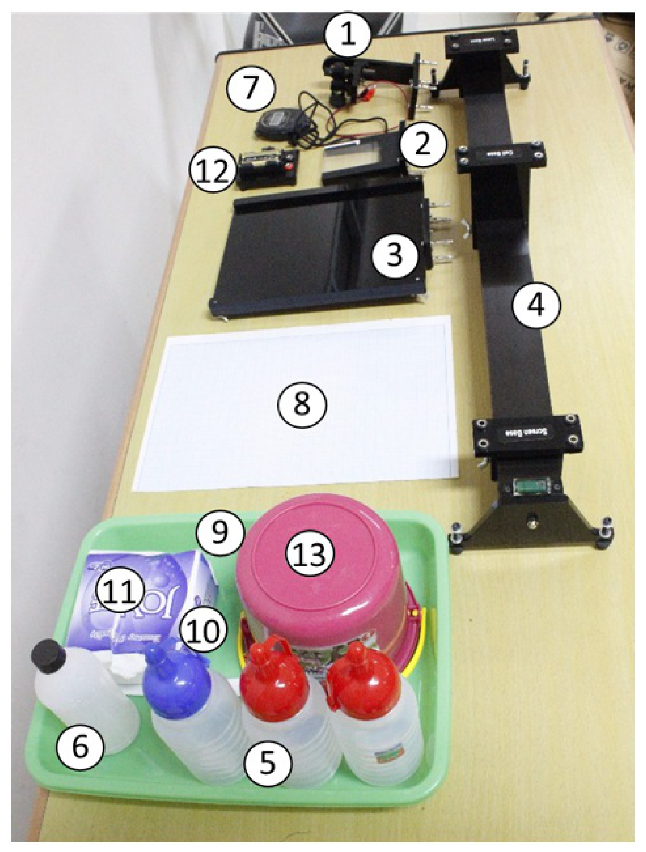
- Line Laser Module (Diode laser with nm and cylindrical lens)
- Diffusion cell (6.5 cm x 0.8 cm x 9.5 cm with holder)
- Screen with holder
- Optical rail with length scale
- Salt-water Solutions
- Distilled Water (Aquadest)
- Stopwatch
- Paper with scale (block millimeter paper)
- Pipette (dropper)
- Knife + Tissue for cleaner
- Tissue
- Battery
- Buckets as waste container of salt and water solution
The schematic diagram of the experimental set-up can be seen in Figure 2.
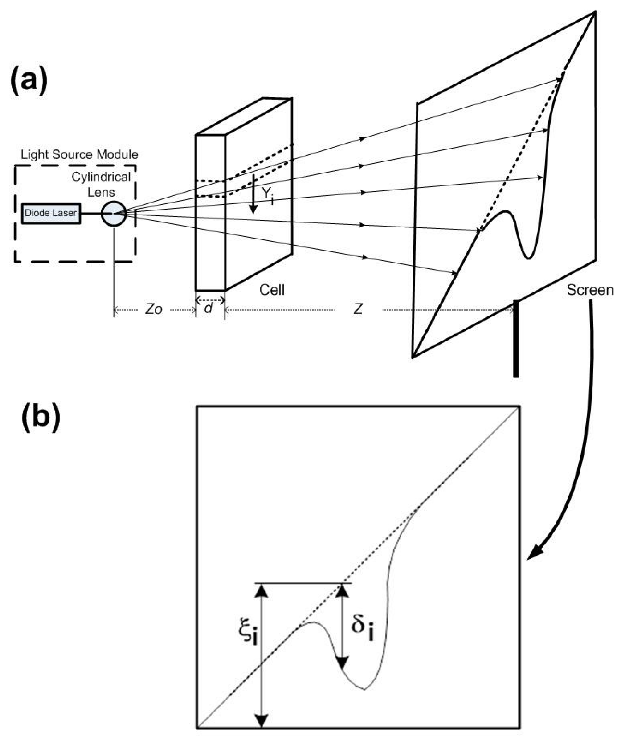
To obtain a profile of the refractive index gradient as a function of vertical position in the fluid we must relate the vertical position on the screen () to the vertical height in the cell (), and relate the vertical deflection () to the gradient of refractive index (). From the geometry of the experimental setup (see Figure 2) we have:
where , and that are shown in Figure 2(a) denote the distance between the light source module and the diffusion cell, the distance between the diffusion cell and the screen, and the diffusion cell's thickness, respectively. For measuring , the line marked on the laser module stand indicates the position of the cylindrical lens.
The thickness of the cell () and the refractive index gradient are both small enough so that the refraction produces negligible vertical displacement of the ray within the cell. In this limit each ray travels at nearly constant vertical height within the cell and is deflected by a single refractive gradient associated with this height.
It can be shown that:
Experimental Procedures
- In order to obtain the deflected laser trace on the screen (as in Figure 2b) you must assemble all the components depicted in Figure 1 by following the schematic shown in Figure 2(a).
- Ensure that the laser is on and its spot and its projection on the screen have diagonal form when it hits perpendicularly the diffusion cell. You may adjust , , and the focal length of the laser (by rotating the back of the laser) in order to obtain a bright and focused line. You can also adjust the direction of the diagonal line on the screw by rotating the laser as a whole (release the laser using the screw on top). In the condition without any water or salt solutions you will see the straight diagonal laser beam.
- Deflected laser trace will appear when the two different solutions are diffusively mixed. Ensure that you pour the salt solution first into the diffusion cell container up to the limit which is marked by white line. Drop the water into the container slowly about 40 drops down the side channel using a pipette, after which you may turn on the stop watch to measure the evolution time of diffusion profile. If the set up of , and the height of the laser are already optimized, the deflected laser trace on the screen will be centered, clear and the depth of the dip as large as possible. You need to find this optimum set-up in order to minimize the error of the measurement.
- After the evolution time of 30 minutes you may draw the laser trace into millimeter block paper attached to the screen using a pencil. Note that in this experiment, you will be asked to do the measurement for 3 different salt solution concentrations (i.e. g/150 ml, g/150 ml and g/150 ml) so that you need to replace the millimeter block frequently. The millimeter block paper should be inserted to the screen and it can be loosen or tighten by rotating the screw attached in the corner of the screen.
- Please make sure that you have written your student code number and the concentration of the solution that you used on this millimeter block paper.
IV. Experiments and Tasks
A: Measurement of Refractive Index Gradient of Salt Water Solution (4.5 points)
You need to perform the steps below for all three salt concentration. Note that no error estimation is needed.
A.1 Perform the experiment to obtain the deflected laser trace on the screen. Duplicate the laser trace into the millimeter block paper attached to the screen using a pencil for evolution time of the diffusion () of 30 minutes. [1,2 т.]
A.2 Measure , , , and (with , are the data points corresponding to different horizontal position) from the laser trace in the millimeter block for evolution time of the diffusion () of 30 minutes. The parameters , , , and are stated in cm. Note that , and are the same for all measurement. Record the results in the Table 1. [1,5 т.]
A.3 Calculate and (with , are the data points for duration time of diffusion () of 30 minutes. Note that , and are the same for all measurement. Record the results in Table 2. Plot vs. for minutes. [1,5 т.]
A.4 Determine the at maximum obtained from question A3. Assign this as . [0,3 т.]
B: Determination of Diffusion Coefficient (4.2 points)
The curves found from question A.3 can be fitted using the following equations:
where , , , , denoted as concentration, initial salt solution concentration, diffusion coefficient, duration time of diffusion, and at maximum of refractive index gradient (), respectively. Note that is constant. The diffusion coefficient can be obtained by using equations (3) and (4) to form a linear relation between and .
B.1 Based on Eqns (3,4), find such functions and that the dependence between and would be linear. [0,9 т.]
B.2 Make a table (Table 3 in the answer sheet) that contains the data points, abscissa axis, ordinate axis of linear equation from B1 for dataset taken from Tasks A. Plot this table. [1,8 т.]
B.3 Determine the diffusion coefficient from linear plot obtained from B2 for data set at minutes. Note that linear dependence may hold only for a subrange of your data. [1,5 т.]
C. Nonlinear diffusion (1.3 points)
C.1 The analysis above is based on the assumption that is independent of . If this is not true, we have so-called nonlinear diffusion. However, near the maximum of we can consider this as an ordinary diffusion, with diffusion coefficient corresponding to the local value of concentration. Determine the rate of change of the diffusion coefficient with the change of salt solution concentration graphically using data from part B. [1,3 т.]
AE1 — Determination of Refractive Index Gradient and Diffusion Coefficient of Salt Solution from Laser Deflection Measurement (10 pt.)
| Student Code | ||||||
|---|---|---|---|---|---|---|
A. Measurement of Refractive Index Gradient of Salt-Water Solution (4.5 pt.)
Question — Answer — Marks
A.1 (1.2 pt.)
Enclose the millimeter block paper that has been used for making the deflectogram. Please make sure that you have written your student code numbers and the concentration of the solutions that you used on this millimeter block paper.
Deflectogram of g/150 mL
Enclose the millimeter block paper that has been used for making the deflectogram. Please make sure that you have written your student code numbers and the concentration of the solutions that you used on this millimeter block paper.
Deflectogram of gr/150 mL
Enclose the millimeter block paper that has been used for making the deflectogram. Please make sure that you have written your student code numbers and the concentration of the solutions that you used on this millimeter block paper.
Deflectogram of g/150 mL
A.2 (1.5 pt.)
Table 1 of g/150 mL
| (cm) | (cm) | (cm) | (cm) | (cm) | |
|---|---|---|---|---|---|
| 1 | |||||
| 2 | ■ | ■ | ■ | ||
| 3 | ■ | ■ | ■ | ||
| 4 | ■ | ■ | ■ | ||
| 5 | ■ | ■ | ■ | ||
| 6 | ■ | ■ | ■ | ||
| 7 | ■ | ■ | ■ | ||
| 8 | ■ | ■ | ■ | ||
| 9 | ■ | ■ | ■ | ||
| 10 | ■ | ■ | ■ | ||
| 11 | ■ | ■ | ■ | ||
| 12 | ■ | ■ | ■ | ||
| 13 | ■ | ■ | ■ | ||
| 14 | ■ | ■ | ■ | ||
| 15 | ■ | ■ | ■ | ||
| 16 | ■ | ■ | ■ | ||
| 17 | ■ | ■ | ■ | ||
| 18 | ■ | ■ | ■ | ||
| 19 | ■ | ■ | ■ | ||
| 20 | ■ | ■ | ■ |
A.3 (1.5 pt.)
Table 2 of g/150 mL
| (cm) | ||
|---|---|---|
| 1 | ||
| 2 | ||
| 3 | ||
| 4 | ||
| 5 | ||
| 6 | ||
| 7 | ||
| 8 | ||
| 9 | ||
| 10 | ||
| 11 | ||
| 12 | ||
| 13 | ||
| 14 | ||
| 15 | ||
| 16 | ||
| 17 | ||
| 18 | ||
| 19 | ||
| 20 |
Plot vs , g/150 mL

Table 2 of g/150 mL
| (cm) | ||
|---|---|---|
| 1 | ||
| 2 | ||
| 3 | ||
| 4 | ||
| 5 | ||
| 6 | ||
| 7 | ||
| 8 | ||
| 9 | ||
| 10 | ||
| 11 | ||
| 12 | ||
| 13 | ||
| 14 | ||
| 15 | ||
| 16 | ||
| 17 | ||
| 18 | ||
| 19 | ||
| 20 |
Plot vs , g/150 mL

Table 2 of g/150 mL
| (cm) | ||
|---|---|---|
| 1 | ||
| 2 | ||
| 3 | ||
| 4 | ||
| 5 | ||
| 6 | ||
| 7 | ||
| 8 | ||
| 9 | ||
| 10 | ||
| 11 | ||
| 12 | ||
| 13 | ||
| 14 | ||
| 15 | ||
| 16 | ||
| 17 | ||
| 18 | ||
| 19 | ||
| 20 |
Plot vs , g/150 mL

A.4 (0.3 pt.)
for 23 g/150 mL = ____ cm
for 28 g/150 mL = ____ cm
for 33 g/150 mL = ____ cm
B: Determination of Diffusion Coefficient (4.2 points)
Question — Answer — Marks
B.1 (0.9 pt.)
Linear form of eq.(3)
B.2 (1.8 pt.)
Table 3 of g/150 mL
| i | ||
|---|---|---|
| 1 | ||
| 2 | ||
| 3 | ||
| 4 | ||
| 5 | ||
| 6 | ||
| 7 | ||
| 8 | ||
| 9 | ||
| 10 | ||
| 11 | ||
| 12 | ||
| 13 | ||
| 14 | ||
| 15 | ||
| 16 | ||
| 17 | ||
| 18 | ||
| 19 | ||
| 20 |
Plot of Table 3, g/150 mL

(slope of the graph) = ____
Table 3 of g/150 mL
| i | ||
|---|---|---|
| 1 | ||
| 2 | ||
| 3 | ||
| 4 | ||
| 5 | ||
| 6 | ||
| 7 | ||
| 8 | ||
| 9 | ||
| 10 | ||
| 11 | ||
| 12 | ||
| 13 | ||
| 14 | ||
| 15 | ||
| 16 | ||
| 17 | ||
| 18 | ||
| 19 | ||
| 20 |
Plot of Table 3, g/150 mL

(slope of the graph) = ____
Table 3 of g/150 mL
| i | ||
|---|---|---|
| 1 | ||
| 2 | ||
| 3 | ||
| 4 | ||
| 5 | ||
| 6 | ||
| 7 | ||
| 8 | ||
| 9 | ||
| 10 | ||
| 11 | ||
| 12 | ||
| 13 | ||
| 14 | ||
| 15 | ||
| 16 | ||
| 17 | ||
| 18 | ||
| 19 | ||
| 20 |
Plot of Table 3, g/150 mL

(slope of the graph) = ____
B.3 (1.5 pt.)
of 23 g/150 mL = ____ cm²/s
of 28 g/150 mL = ____ cm²/s
of 33 g/150 mL = ____ cm²/s
C. Nonlinear diffusion (1.3 points)
Question — Answer — Marks
C.1 (1.3 pt.)
Plot vs.

The rate change of diffusion coefficient w.r.t the change of salt solution concentrations:
Отговори
The official sample key gives h = (1.5 ± 0.1) cm for each concentration. D is (1.38–1.58)×10⁻⁵, (1.26–1.46)×10⁻⁵ and (1.03–1.23)×10⁻⁵ cm²/s for 23, 28 and 33 g/150 mL respectively. dD/dc is −4.2×10⁻⁵ till −15.8×10⁻⁵ cm² mL g⁻¹ s⁻¹.
These are the printed official sample results and marking ranges. Individual measured data may differ.
Решение
E1. Marking Scheme & Solution
Determination of Refractive Index Gradient and Diffusion Coefficient of Salt Solution from Laser Deflection Measurement (10 points)
A. Measurement of Refractive Index Gradient of Salt Water Solution (4.5 points)
A.1 Deflectogram of g/150 mL
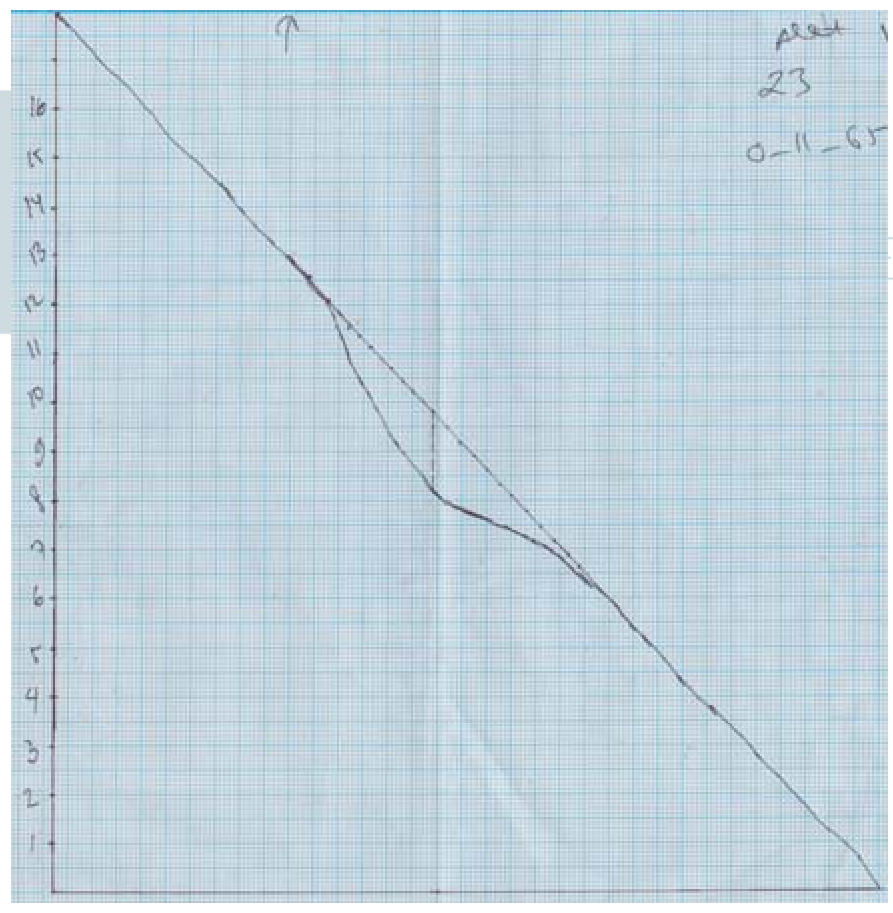
Centred
Depth of dip: 1.5 - 1.6 cm (0.4 pts)
| Answer | Marks |
|---|---|
| No dip | -0.4 |
| No reference line | -0.05 |
| Deflectogram (DL) not at the centre (+- 5mm) but the depth of dip still in 1.5 - 1.6 cm range | -0.05 |
| DL at the centre, the depth of dip <1.5 cm or >1.6 cm | -0.05 |
| DL not at the centre, the depth of dip <1.5 cm or >1.6 cm | -0.1 |
Deflectogram of gr/150 mL
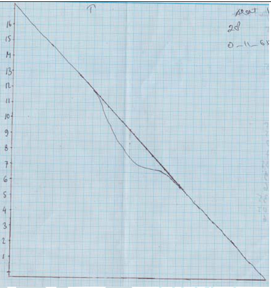
Centred
Deep of dip: 1.7 - 1.9 cm (0.4 pts)
| Answer | Marks |
|---|---|
| No dip | -0.4 |
| No reference line | -0.05 |
| Deflectogram (DL) not at the centre (+- 5mm) but the depth of dip still in 1.7 cm - 1.9 cm range | -0.05 |
| DL at the centre, the depth of dip <1.7 cm or >1.9 cm | -0.05 |
| DL not at the centre, the depth of dip <1.7 cm or >1.9 cm | -0.1 |
Deflectogram of g/150 mL
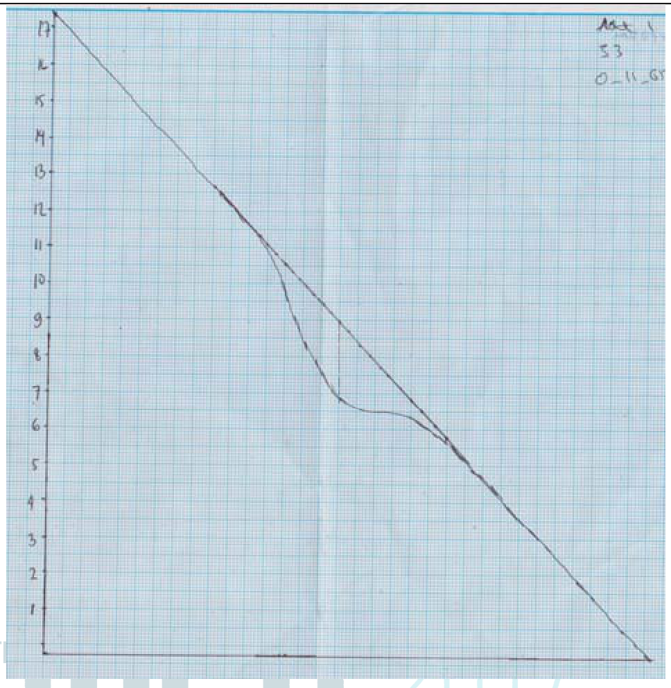
Deep of dip: 1.9 - 2.3 cm (0.4 pts)
| Answer | Marks |
|---|---|
| No dip | -0.4 pts |
| No reference line | -0.05 pts |
| Deflectogram (DL) not at the centre (+-5mm) but the depth of dip still in 1.9 - 2.3 cm range | -0.05 pts |
| DL at the centre, the depth of dip <1.9 cm or >2.3 cm | -0.05 pts |
| DL not at the centre, the depth of dip <1.9 cm or >2.3 cm | -0.1 |
A.2 Table 1 of g/150 mL
| (cm) | (cm) | (cm) | (cm) | (cm) | |
|---|---|---|---|---|---|
| 1 | 0.05 | 11.55 | |||
| 2 | 0.35 | 11.3 | |||
| 3 | 0.6 | 11.05 | |||
| 4 | 0.9 | 10.85 | |||
| 5 | 1 | 10.65 | |||
| 6 | 1.1 | 10.35 | |||
| 7 | 1.3 | 10.15 | |||
| 8 | 1.4 | 9.85 | |||
| 9 | 1.45 | 9.7 | |||
| 10 | 1.5 | 9.45 | |||
| 11 | 1.6 | 9.25 | |||
| 12 | 1.5 | 8.95 | |||
| 13 | 1.4 | 8.65 | |||
| 14 | 1.2 | 8.35 | |||
| 15 | 1 | 8.05 | |||
| 16 | 0.8 | 7.75 | |||
| 17 | 0.7 | 7.55 | |||
| 18 | 0.5 | 7.25 | |||
| 19 | 0.3 | 6.95 | |||
| 20 | 0.2 | 6.65 | |||
| 21 | 0.05 | 6.4 |
Marks
Optimum and
# data = 20
(0.5 pts)
Correct data point must be extracted from deflectogram
| Answer | Marks |
|---|---|
| # correct data points >= 20, but not all observable (, , ) are written | -0.05 pts |
| Incorrect | -0.05 pts |
| 15 <= # correct data points < 20, | -0.15 pts |
| 10 < # correct data points < 15 | -0.3 pts |
| # correct data points < 10 | -0.45 pts |
Table 1 of g/150 mL
| (cm) | (cm) | (cm) | (cm) | (cm) | |
|---|---|---|---|---|---|
| 1 | 0.05 | 11.65 | |||
| 2 | 0.25 | 11.4 | |||
| 3 | 0.4 | 11.2 | |||
| 4 | 0.8 | 11 | |||
| 5 | 1 | 10.75 | |||
| 6 | 1.2 | 10.4 | |||
| 7 | 1.4 | 10.2 | |||
| 8 | 1.5 | 10 | |||
| 9 | 1.6 | 9.8 | |||
| 10 | 1.7 | 9.5 | |||
| 11 | 1.75 | 9.25 | |||
| 12 | 1.7 | 8.95 | |||
| 13 | 1.65 | 8.7 | |||
| 14 | 1.5 | 8.4 | |||
| 15 | 1.25 | 8.05 | |||
| 16 | 0.9 | 7.6 | |||
| 17 | 0.6 | 7.3 | |||
| 18 | 0.4 | 7.05 | |||
| 19 | 0.25 | 6.75 | |||
| 20 | 0.05 | 6.3 |
Marks
Optimum and
# data = 20
(0.5 pts)
Correct data point must be extracted from deflectogram
| Answer | Marks |
|---|---|
| # correct data points >= 20, but not all observable (, , ) are written | -0.05 pts |
| Incorrect | -0.05 pts |
| 15 <= # correct data points < 20, | -0.15 pts |
| 10 < # correct data points < 15 | -0.3 pts |
| # correct data points < 10 | -0.45 pts |
Table 1 of g/150 mL
| (cm) | (cm) | (cm) | (cm) | (cm) | |
|---|---|---|---|---|---|
| 1 | 0.05 | 11.6 | |||
| 2 | 0.15 | 11.4 | |||
| 3 | 0.35 | 11.1 | |||
| 4 | 0.65 | 10.85 | |||
| 5 | 1.1 | 10.6 | |||
| 6 | 1.3 | 10.4 | |||
| 7 | 1.5 | 10.2 | |||
| 8 | 1.7 | 10 | |||
| 9 | 1.85 | 9.7 | |||
| 10 | 2 | 9.5 | |||
| 11 | 2.1 | 9.25 | |||
| 12 | 2 | 9 | |||
| 13 | 1.8 | 8.6 | |||
| 14 | 1.5 | 8.3 | |||
| 15 | 1.25 | 8.05 | |||
| 16 | 1 | 7.8 | |||
| 17 | 0.75 | 7.45 | |||
| 18 | 0.55 | 7.15 | |||
| 19 | 0.4 | 6.8 | |||
| 20 | 0.2 | 6.4 | |||
| 21 | 0.05 | 6.1 |
Marks
# data point >= 20
(0.5 pts)
Correct data point must be extracted from deflectogram
| Answer | Marks |
|---|---|
| # correct data points >= 20, but not all observable (, , ) are written | -0.05 pts |
| Incorrect | -0.05 pts |
| 15 <= # correct data points < 20, | -0.15 pts |
| 10 < # correct data points < 15 | -0.3 pts |
| # correct data points < 10 | -0.45 pts |
A.3 Table 2 of g/150 mL.
| (cm) | ||
|---|---|---|
| 1 | 1.85944 | 0.00117 |
| 2 | 1.81919 | 0.00819 |
| 3 | 1.77894 | 0.01404 |
| 4 | 1.74674 | 0.02106 |
| 5 | 1.71455 | 0.02340 |
| 6 | 1.66625 | 0.02574 |
| 7 | 1.63405 | 0.03043 |
| 8 | 1.58575 | 0.03277 |
| 9 | 1.56161 | 0.03394 |
| 10 | 1.52136 | 0.03511 |
| 11 | 1.48916 | 0.03745 |
| 12 | 1.44086 | 0.03511 |
| 13 | 1.39257 | 0.03277 |
| 14 | 1.34427 | 0.02809 |
| 15 | 1.29597 | 0.02340 |
| 16 | 1.24767 | 0.01872 |
| 17 | 1.21548 | 0.01638 |
| 18 | 1.16718 | 0.01170 |
| 19 | 1.11888 | 0.00702 |
| 20 | 1.07058 | 0.00468 |
| 21 | 1.03034 | 0.00117 |
# data = 20 (0.25 pts)
Jury must check the data in table
| Answer | Marks |
|---|---|
| # wrong data point < 3 | -0 |
| 3 < # wrong data point < 6 | -0.05 pts |
| # wrong data point > 6 | -0.25 pts |
Plot vs . g/150 mL.
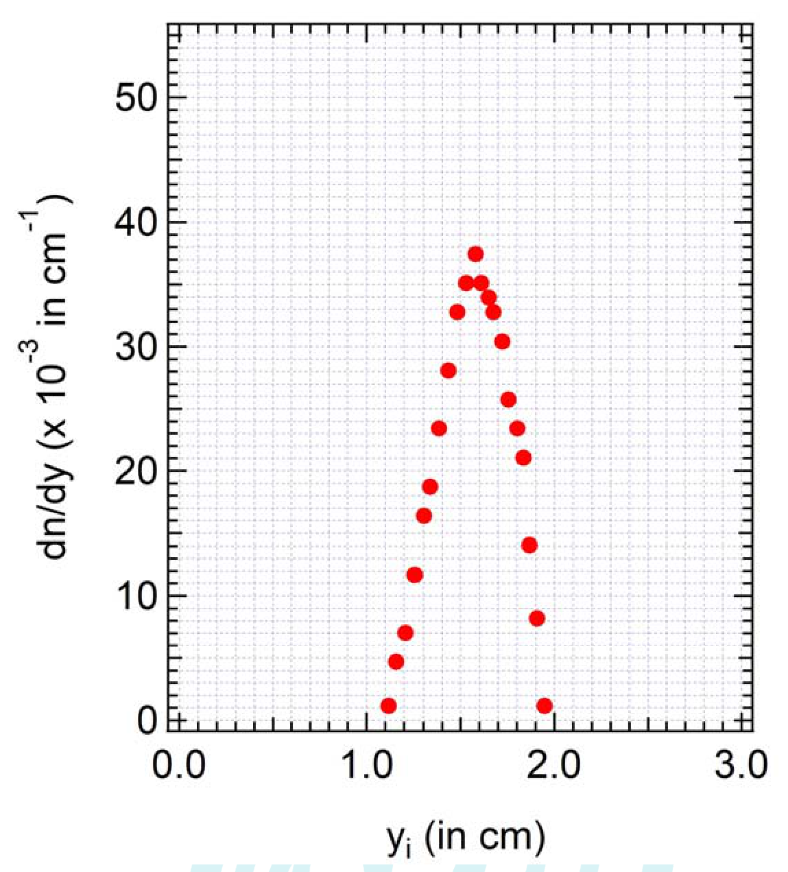
“Gaussian-Like” shape
(0.25 pts)
Answer column (printed order)
- No x-axis label
- No x-axis unit
- Without x-axis unit
- No y-axis label
- No y-axis unit
- Without y-axis unit
- Ordinate axis represented in 2 digid behind point
- Ordinate axis represented in 3 digid behind point
- Random shape
Marks column (printed order)
- -0.01 pts
- -0.01 pts
- -0.01 pts
- -0.01 pts
- -0.01 pts
- -0.01 pts
- -0.05 pts
- -0 pts
- -0.25 pts
Table 2 of g/150 mL.
| (cm) | ||
|---|---|---|
| 1 | 1.87554 | 0.00117 |
| 2 | 1.83529 | 0.00585 |
| 3 | 1.80309 | 0.00936 |
| 4 | 1.77089 | 0.01872 |
| 5 | 1.73065 | 0.02340 |
| 6 | 1.67430 | 0.02809 |
| 7 | 1.64210 | 0.03277 |
| 8 | 1.60990 | 0.03511 |
| 9 | 1.57770 | 0.03745 |
| 10 | 1.52941 | 0.03979 |
| 11 | 1.48916 | 0.04096 |
| 12 | 1.44086 | 0.03979 |
| 13 | 1.40061 | 0.03862 |
| 14 | 1.35232 | 0.03511 |
| 15 | 1.29597 | 0.02926 |
| 16 | 1.22352 | 0.02106 |
| 17 | 1.17523 | 0.01404 |
| 18 | 1.13498 | 0.00936 |
| 19 | 1.08668 | 0.00585 |
| 20 | 1.01424 | 0.00117 |
# data = 20 (0.25 pts)
Jury must check the data in table
| Answer | Marks |
|---|---|
| # wrong data point < 3 | -0 |
| 3 < # wrong data point < 6 | -0.05 pts |
| # wrong data point > 6 | -0.25 pts |
Plot vs . g/150 mL.
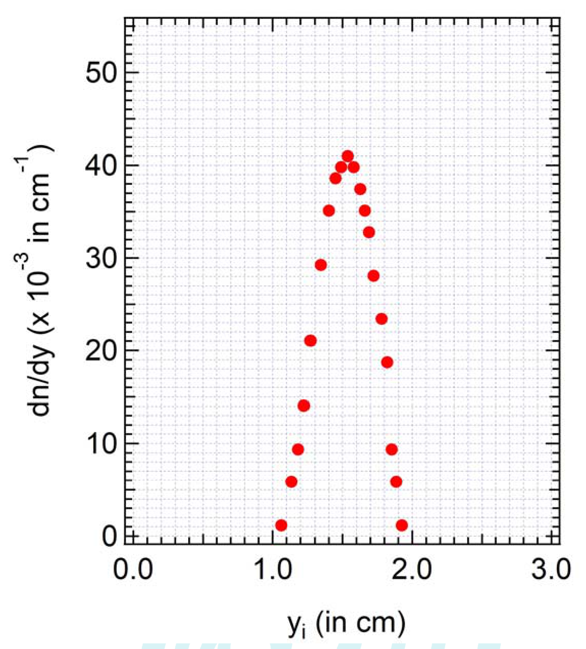
“Gaussian-Like” shape
(0.25 pts)
Answer column (printed order)
- without x-axis label
- without x-axis unit
- wrong x-axis unit
- without y-axis label
- without y-axis unit
- wrong y-axis unit
- Ordinate axis represented in 2 digid behind point
- Ordinate axis represented in 3 digid behind point
- Random shape of the curve
Marks column (printed order)
- -0.01 pts
- -0.01 pts
- -0.01 pts
- -0.01 pts
- -0.01 pts
- -0.01 pts
- -0.05 pts
- -0 pts
- -0.25 pts
Table 2 of g/150 mL.
| (cm) | ||
|---|---|---|
| 1 | 1.86749 | 0.00117 |
| 2 | 1.83529 | 0.00351 |
| 3 | 1.78699 | 0.00819 |
| 4 | 1.74674 | 0.01521 |
| 5 | 1.70650 | 0.02574 |
| 6 | 1.67430 | 0.03043 |
| 7 | 1.64210 | 0.03511 |
| 8 | 1.60990 | 0.03979 |
| 9 | 1.56161 | 0.04330 |
| 10 | 1.52941 | 0.04681 |
| 11 | 1.48916 | 0.04915 |
| 12 | 1.44891 | 0.04681 |
| 13 | 1.38452 | 0.04213 |
| 14 | 1.33622 | 0.03511 |
| 15 | 1.29597 | 0.02926 |
| 16 | 1.25572 | 0.02340 |
| 17 | 1.19938 | 0.01755 |
| 18 | 1.15108 | 0.01287 |
| 19 | 1.09473 | 0.00936 |
| 20 | 1.03034 | 0.00468 |
| 21 | 0.98204 | 0.00117 |
# data = 20 (0.25 pts)
Jury must check the data in table
| Answer | Marks |
|---|---|
| # wrong data point < 3 | -0 |
| 3 < # wrong data point < 6 | -0.05 pts |
| # wrong data point > 6 | -0.25 pts |
Plot vs . g/150 mL.
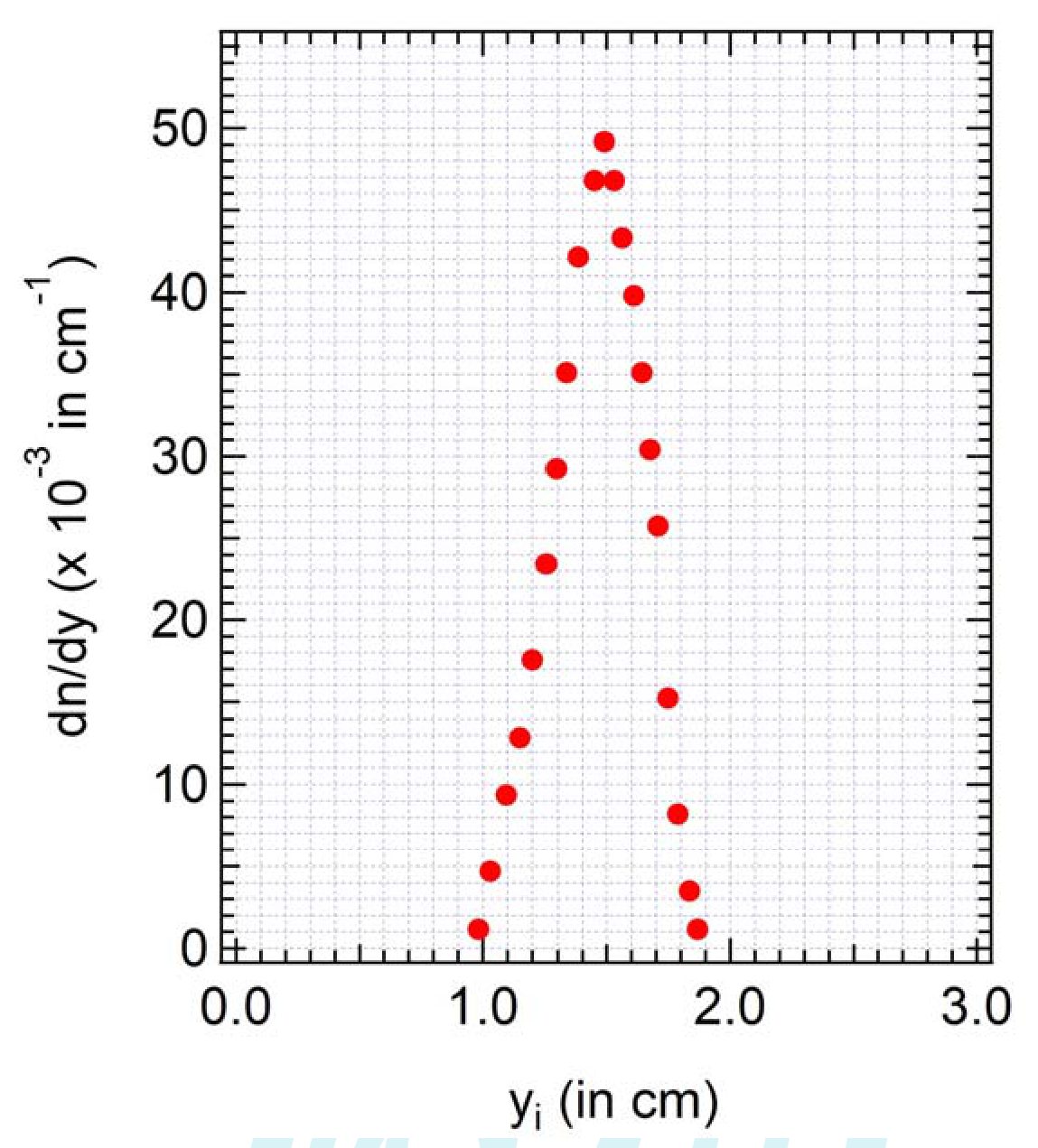
(0.25 pts)
Answer column (printed order)
- without x-axis label
- without x-axis unit
- wrong x-axis unit
- without y-axis label
- without y-axis unit
- wrong y-axis unit
- Ordinate axis represented in 2 digid behind point
- Ordinate axis represented in 3 digid behind point
- Random shape of the curve
Marks column (printed order)
- -0.01 pts
- -0.01 pts
- -0.01 pts
- -0.01 pts
- -0.01 pts
- -0.01 pts
- -0.05 pts
- -0 pts
- -0.25 pts
A.4
| Answer | Marks |
|---|---|
| for 23 g/150 mL = cm | 0.1 pts |
| for 28 g/150 mL = cm | 0.1 pts |
| for 33 g/150 mL = cm | 0.1 pts |
| Answer | Marks |
|---|---|
| If is correctly determined from graph A3 for each concentration | -0 |
| If is not correctly determined from graph A3 for each concentration | -0.1 |
B: Determination of Diffusion Coefficient (4.2 points)
B.1 Linear form of eq.(3)
0.9 pt
Constant:
| Answer | Marks |
|---|---|
| Other than (b1) | -0.9 pts |
B.2 Table 3 of g/150 mL.
| i | ||
|---|---|---|
| 1 | 0.06592 | -3.86003 |
| 2 | 0.050423 | -3.75467 |
| 3 | 0.031065 | -3.65936 |
| 4 | 0.020752 | -3.4923 |
| 5 | 0.00917 | -3.41819 |
| 6 | 0.005128 | -3.3831 |
| 7 | 0.000984 | -3.3492 |
| 8 | 6.99E-07 | -3.28466 |
| 9 | 0.002414 | -3.3492 |
| 10 | 0.009493 | -3.41819 |
| 11 | 0.021237 | -3.57235 |
| 12 | 0.037646 | -3.75467 |
| 13 | 0.05872 | -3.97781 |
# data = 10 (0.3 pts)
Jury must check the data in table
| Answer | Marks |
|---|---|
| # of data point > 10 | -0 pts |
| 3 <= # of data point < 10 | -0.05 pts |
| # of data point < 3 | -0.3 pts |
| # wrong data point < 3 | -0 |
| 3 < # wrong data point < 6 | -0.05 pts |
| # wrong data point > 6 | -0.25 |
Plot of Table 3. g/150 mL.
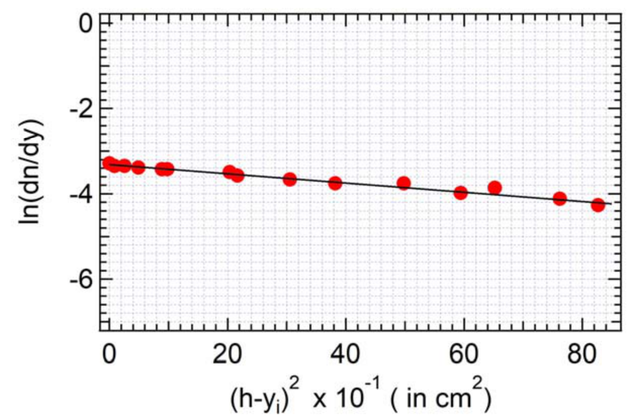
# data = 10 (0.3 pts)
Using linear regression of eq. (B1.1), we obtain
(slope) = till
Answer column (printed order)
- without x-axis label
- without x-axis unit
- wrong x-axis unit
- without y-axis label
- without y-axis unit
- wrong y-axis unit
of data point in linear range > 10
- 3 <= # of data point in linear range < 10
of data point in linear range < 3 or random shape of curve
- m is out of range
Marks column (printed order)
- -0.01 pts
- -0.01 pts
- -0.01 pts
- -0.01 pts
- -0.01 pts
- -0.01 pts
- -0 pts
- -0.05 pts
- -0.25 pts
- -0.3 pts
Table 3 of g/150 mL.
| i | ||
|---|---|---|
| 1 | 0.057912 | -3.75467 |
| 2 | 0.033968 | -3.57235 |
| 3 | 0.023136 | -3.41819 |
| 4 | 0.014378 | -3.3492 |
| 5 | 0.007693 | -3.28466 |
| 6 | 0.001553 | -3.22404 |
| 7 | 6.99E-07 | -3.19505 |
| 8 | 0.002414 | -3.22404 |
| 9 | 0.007989 | -3.25389 |
| 10 | 0.018955 | -3.3492 |
| 11 | 0.037646 | -3.53152 |
| 12 | 0.071007 | -3.86003 |
| 13 | 0.099079 | -4.26549 |
# data = 10 (0.3 pts)
Jury must check the data in table
| Answer | Marks |
|---|---|
| # of data point > 10 | -0 pts |
| 3 <= # of data point < 10 | -0.05 pts |
| # of data point < 3 | -0.3 pts |
| # wrong data point < 3 | -0 |
| 3 < # wrong data point < 6 | -0.05 pts |
| # wrong data point > 6 | -0.25 |
Plot of Table 3. g/150 mL.
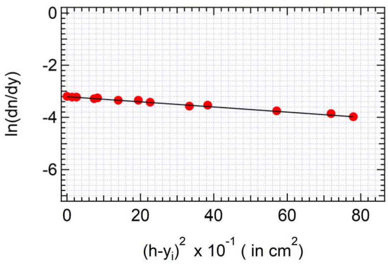
# data = 10 (0.3 pts)
Using linear regression of eq. (B1.1), we obtain
(slope) = till
Answer column (printed order)
- without x-axis label
- without x-axis unit
- wrong x-axis unit
- without y-axis label
- without y-axis unit
- wrong y-axis unit
of data point in linear range > 10
- 3 <= # of data point in linear range < 10
of data point in linear range < 3 or random shape of curve
- m is out of range
Marks column (printed order)
- -0.01 pts
- -0.01 pts
- -0.01 pts
- -0.01 pts
- -0.01 pts
- -0.01 pts
- -0 pts
- -0.05 pts
- -0.3 pts
- -0.3 pts
Table 3 of g/150 mL.
| i | ||
|---|---|---|
| 1 | 0.046873 | -3.65936 |
| 2 | 0.033968 | -3.4923 |
| 3 | 0.023136 | -3.3492 |
| 4 | 0.014378 | -3.22404 |
| 5 | 0.005128 | -3.13948 |
| 6 | 0.001553 | -3.06152 |
| 7 | 6.99E-07 | -3.01273 |
| 8 | 0.001688 | -3.06152 |
| 9 | 0.011126 | -3.16688 |
| 10 | 0.023647 | -3.3492 |
| 11 | 0.037646 | -3.53152 |
| 12 | 0.054884 | -3.75467 |
| 13 | 0.08446 | -4.04235 |
# data = 10 (0.3 pts)
Jury must check the data in table
| Answer | Marks |
|---|---|
| # of data point > 10 | -0 pts |
| 3 <= # of data point < 10 | -0.05 pts |
| # of data point < 3 | -0.3 pts |
| # wrong data point < 3 | -0 |
| 3 < # wrong data point < 6 | -0.05 pts |
| # wrong data point > 6 | -0.25 |
Plot of Table 3. g/150 mL.
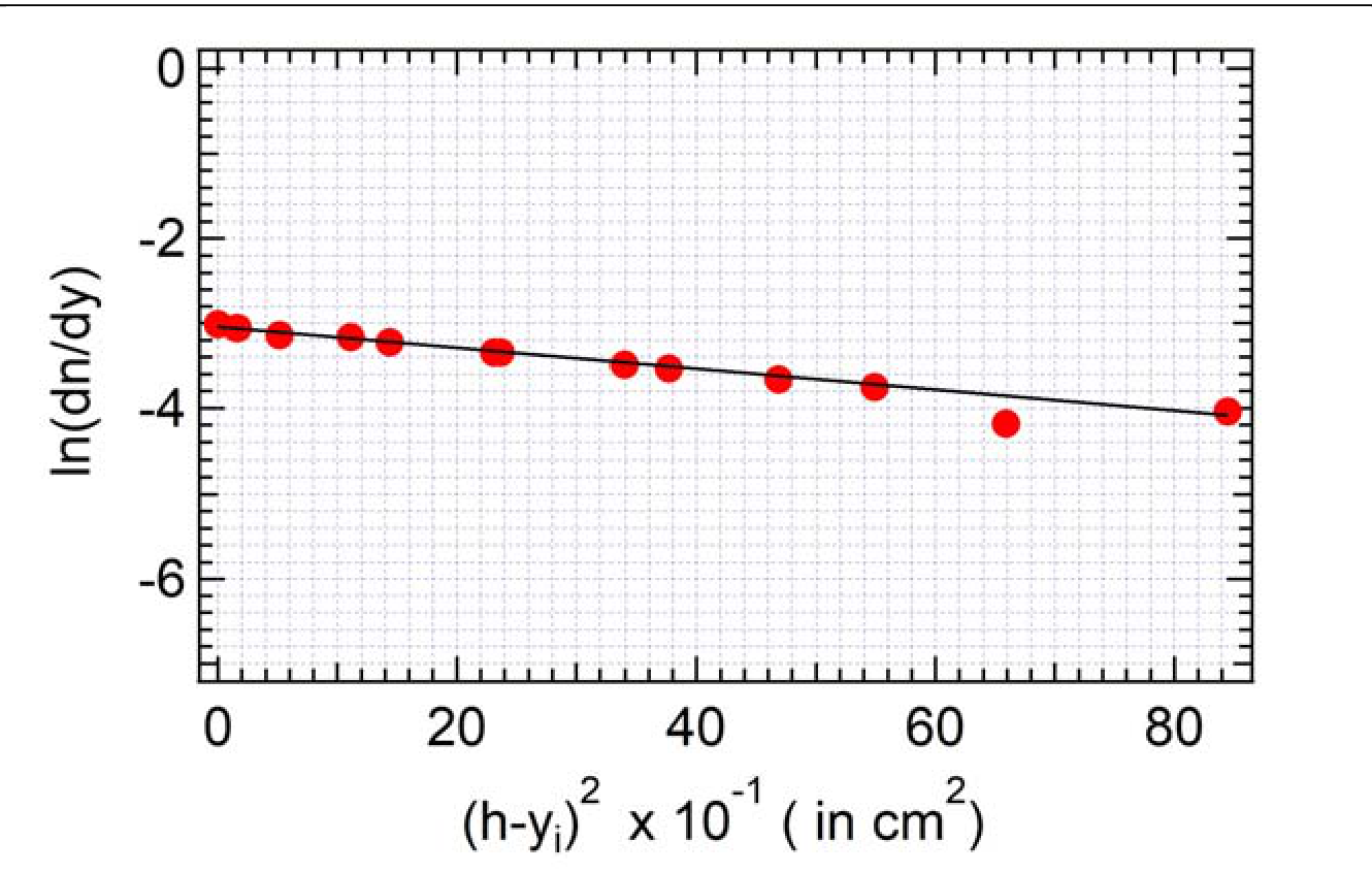
# data = 10 (0.3 pts)
Using linear regression of eq. (B1.1), we obtain
(slope) = till
Answer column (printed order)
- without x-axis label
- without x-axis unit
- wrong x-axis unit
- without y-axis label
- without y-axis unit
- wrong y-axis unit
- m is out of range
of data point in linear range > 10
- 3 <= # of data point in linear range < 10
of data point in linear range < 3 or random shape of curve
Marks column (printed order)
- -0.01 pts
- -0.01 pts
- -0.01 pts
- -0.01 pts
- -0.01 pts
- -0.01 pts
- -0.3 pts
- -0 pts
- -0.05 pts
- -0.3 pts
B.3
| Answer | Marks |
|---|---|
| of 23 g/150 mL = | 0.5 pts |
| of 28 g/150 mL = | 0.5 pts |
| of 33 g/150 mL = | 0.5 pts- |
| Answer | Marks |
|---|---|
| is out of range for each concentration | -0.5 pts |
C. Nonlinear diffusion (1.3 points)
C.1 Plot vs.
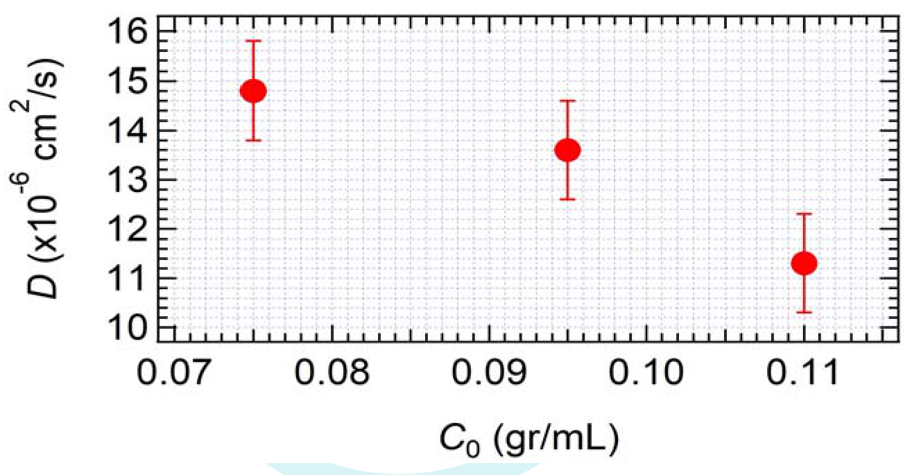
0.8 pts
| Answer | Marks |
|---|---|
| Without error bars | -0 |
| Value of not stated in | -0.4 pts |
0.5 pts
| Answer | Marks |
|---|---|
| Without or wrong unit | -0.01 pts |
| Out of range | -0.5 pts |
Теми и трудност
Оценена трудност: 4/5.
Оптика · Топлинни явления · Пречупване · Молекулно-кинетична теория
Предпоставки: Гимназиална подготовка, Разширена олимпиадна подготовка
Оригинал в Архива: exp1.pdf · официални решения: exp1_sol.pdf · допълнителни данни: exp1_anssheet.pdf · допълнителни данни: exp_instructions.pdf