Съдържание
УсловиеA. IntroductionB. Apparatus[1] Determination of the magnet's magnetization () (2.5 pt.)[2] The Magnetic Levitation effect and Magnetic Susceptibility () (1 pt.)[3] The camelback potential oscillation and magnetic susceptibility () (1 pts)[4] Oscillator quality factor () and estimate of air viscosity (3 pt.)[5] PDL Trap Seismometer (0.5 pt.)[6] PDL Trap Tiltmeter (2 pt.)AE2 — Parallel Dipole Line Magnetic Trap for Earthquake & Volcanic Sensing (10 points)ОтговориРешениеIPhO 2017, Експеримент — Задача 2. Parallel Dipole Line Magnetic Trap for Earthquake and Volcanic Sensing
Parallel Dipole Line Magnetic Trap for Earthquake and Volcanic Sensing · 18 юли 2017 г. · 10 т.
Внимание: Бележка към темата
The original official key prints a missing minus sign in the second expression for χ in A.9 and the impossible marking interval 22.8 < D < 22.2 cm in B.4. The original answer sheet labels division 4 as 4.0 points; the question and key give 3 points. These printed inconsistencies are preserved.
General instructions: Experimental Examination
July 18, 2017
The experimental examination lasts for 5 hours and is worth a total of 20 points.
Before the exam
- You must not open the envelopes containing the problems before the sound signal indicating the beginning of the examination.
- The beginning and end of the examination will be indicated by a sound signal. There will be announcements every hour indicating the elapsed time, as well as fifteen minutes before the end of the examination (before the final sound signal).
During the exam
- Dedicated answer sheets are provided for writing your answers. Enter the observations into the appropriate tables, boxes or graphs in the corresponding answer sheet. For every problem, there are work sheets for carrying out detailed work. Be sure to always use the work sheets that belong to the problem you are currently working on (check the problem number in the header). If you have written something on any sheet which you do not want to be graded, cross it out. Only use the front side of every page. Do not forget to put your student code numbers in each working sheets or answer sheets in the field provided. Answers or working results will not be graded if there is no student code numbers written.
- In your answers, try to be as concise as possible: use equations, logical operators and sketches to illustrate your thoughts whenever possible. Avoid the use of long sentences.
- Explicit error calculation is not required unless explicitly asked for. However, you are asked to give an appropriate number of significant digits when stating numbers. Also, you should decide on the appropriate number of data points or measurement repetitions unless specific instructions are given.
- You may often be able to solve later parts of a problem without having solved the previous ones.
- You are not allowed to leave your working place without permission. If you need any assistance (need to refill your drinking water bottle, broken calculator, need to visit a restroom, etc.), please draw the attention of a supervisor by lifting one of the three flags into the air ("Refill my water bottle, please", "I need to go to the toilet, please", or "I need help, please" in all other cases).
At the end of the exam
- At the end of the examination you must stop writing immediately.
- For every problem, sort the corresponding sheets in the following order: questions, answer sheets, work sheets.
At the end of the exam — continued
- For E1 (Experimental Problem No. 1) you need to enclose the millimeter block paper that has been used for making the deflactogram. Please make sure that you have written your student code numbers and the concentration of the solutions that you used on this millimeter block paper.
- You must write the number and total number of pages used on your working sheets at the bottom of each pages.
- Put all the sheets belonging to one problem into the same envelope. Also put the general instructions into the remaining separate envelope (if available or just put in outside the envelope if remaining separate envelope is not available). Also hand in empty sheets. You are not allowed to take any sheets of paper out of the examination area.
- Leave your writing equipment (provided by the committee, if any) as well as the provided calculator on the experiment table.
- Wait at your table until your envelopes and all the necessary equipment are collected. Once all envelopes and equipment are collected, your guide will escort you out of the examination area. Don’t forget to take your water bottle with you or your remaining snack.
Условие
A. Introduction
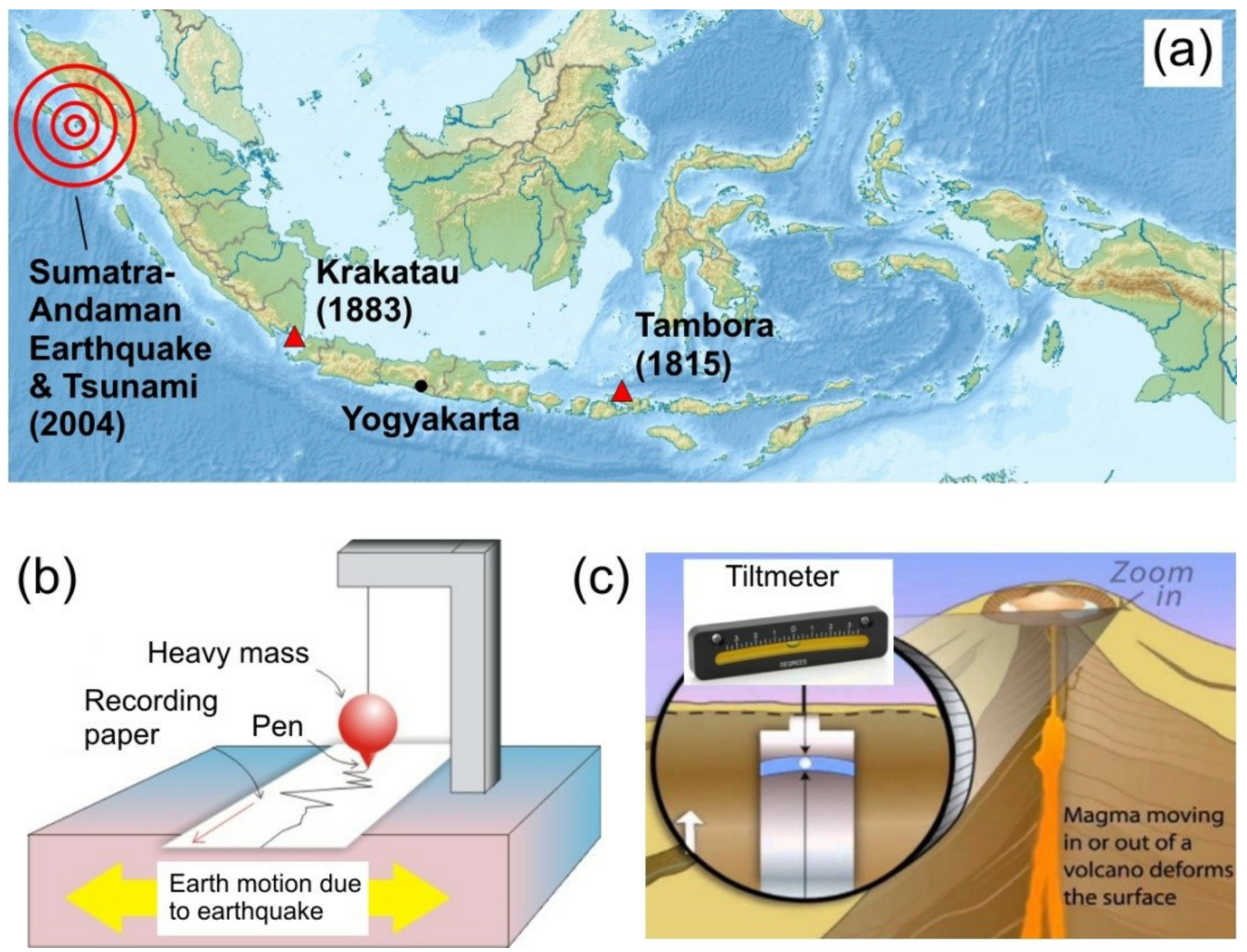
Indonesia is the world's largest archipelago, with about 17,000 islands sprawling in the tropics and thus often called "the jewel of the equator". Unfortunately, it has plenty of natural threats such as earthquake and volcanic eruptions. Colossal catastrophic events (Fig. 1a) such as the Sumatra-Andaman earthquake and tsunami (2004), Krakatau (1883) and Tambora (1815) volcanic eruptions are among the deadliest disasters in the recorded history of the world. To detect earthquake, we use a seismometer, usually a pendulum-based system to measure the ground displacement or acceleration (Fig. 1b). To monitor volcano, we use tiltmeter to detect a change in ground inclination due to underground magma movement (Fig. 1c). In this problem we will explore the physics and applications of a new kind of magnetic trap and sensor - called Parallel Dipole Line (PDL) trap system - for sensing earthquake and to monitor volcano.
Parallel dipole line system is an arrangement of two linear distribution of magnetic dipole (also called a dipole line) as shown in Fig. 2. Recently two Indonesian physicists discovered a very interesting effect in this system: if the length of the dipole line is longer than certain critical length the magnetic field becomes stronger on the edges which produces a "camelback potential" as shown in Fig. 2a.* This "camelback effect" is important as it enables this system to serve as a new type of magnetic trap called Parallel Dipole Line (PDL) trap. Experimentally we can realize this PDL trap using a pair of diametric magnets i.e. a cylinder magnets with magnetization along diameter as shown in Fig. 2c where the north and south poles are on the curved sides instead of the flat faces.
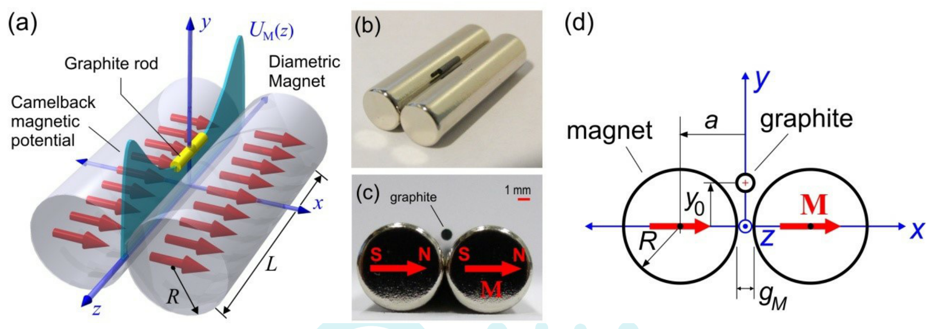
If we drop a graphite rod (ordinary pencil lead) into the trap it will levitate or gets trapped in a stable condition. This occurs because in -direction the graphite is repelled by the magnets from both sides and in vertical () direction the magnetic repulsion force balance the gravity making it levitates at height (Fig. 2d). In longitudinal direction () the camelback potential holds the graphite stable.
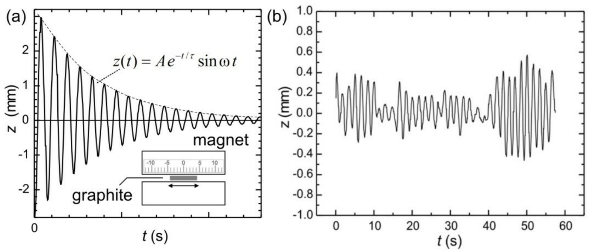
The camelback potential of the magnetic trap serves as a one-dimensional oscillator. If you give a little perturbation along the -axis to the graphite rod, it will exhibit underdamped oscillation as shown in Fig. 3a. This PDL trap can be used as a sensitive seismometer. If the ground underneath shakes, the graphite rod tends to remain stable and its relative displacement (Fig. 3b) is the "earthquake" signal. Similarly, it can also be used as sensitive tiltmeter: if you tilt the trap slightly, the graphite rod will move significantly without any friction.
We will now investigate the physics and application of this PDL trap in two sections.
Section A: Basic characteristics
(1) Determination of the magnet's magnetization (2.5 pt.)
(2) Magnetic levitation and magnetic susceptibility (1.0 pt.)
(3) The camelback potential oscillation and magnetic susceptibility (1.0 pt.)
(4) Oscillator quality factor and determination of air viscosity (3.0 pt.)
Section B: Applications
(5) PDL Trap Seismometer (0.5 pt.)
(6) PDL Trap Tiltmeter (2.0 pt.)
B. Apparatus
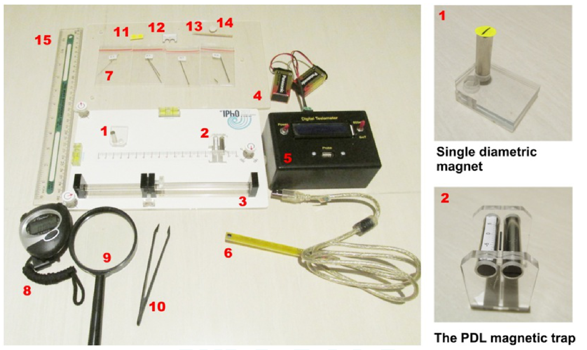
- Single diametric magnet assembly. Yellow sticker is attached to mark magnetization.
- The PDL magnetic trap assembly, shown with levitating graphite. Please do not remove the magnets from the assembly.
- Top platform with 3 screws
- Bottom platform
- Tesla meter to measure magnetic field. Batteries are provided to power up the Tesla meter and a cable to connect the Hall probe to Tesla meter.
- Hall sensor probe of the Tesla meter
- Graphite rods (pencil leads) with 4 diameter sizes HB/0.3, HB/0.5, HB/0.7, and HB/0.9. See the constants and data for exact diameters. You may need to break these graphite rods to specific lengths as required.
- Stopwatch
- Magnifying glass
- Tweezer, anti-static
- Round yellow sticker—to mark the magnetization direction (north-south pole) of single magnet
- "Insert-ruler" to measure graphite levitation height
- Toothpick to move around the graphite rod
- Silly putty to stick magnet assemblies to platform
- Ruler
INSTRUCTIONS & WARNING:
- Keep the single magnet and the PDL trap (double magnet) assemblies away from each other. They can hit each other and crack!
- Turn off the Tesla meter if not in use to save battery!
- Please detach items 7, 11-14 carefully from bottom platform (item 4) and then place the top platform (item 3) on the bottom platform.
- You can use the three screws to adjust the level of the top platform.
CONSTANTS AND DATA:
| Radius of the diametric magnet | 3.2 mm | |
| Length of the diametric magnet | 25.4 mm | |
| Gap of the PDL trap | 1.5 mm | |
| Mass density of graphite | 1680 kg/m³ | |
| Graphite rod "HB/0.3" diameter | 0.38 mm | |
| Graphite rod "HB/0.5" diameter | 0.56 mm | |
| Graphite rod "HB/0.7" diameter | 0.70 mm | |
| Graphite rod "HB/0.9" diameter | 0.90 mm | |
| Room temperature | 298 K | |
| Magnetic permeability in vacuum | ||
| Boltzmann constant | ||
| Acceleration of gravity | 9.8 m/s² |
[1] Determination of the magnet's magnetization () (2.5 pt.)
C. Experiment & Questions
SECTION A. BASIC CHARACTERISTICS OF THE PDL TRAP
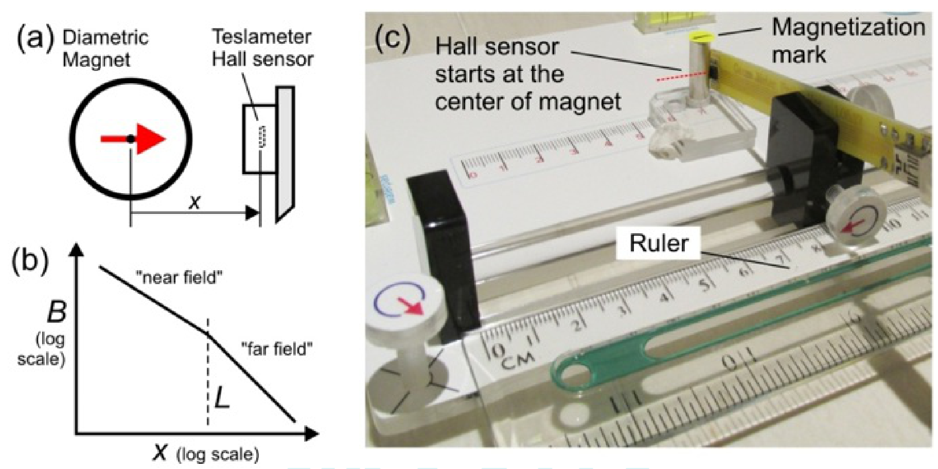
The strength of the magnetic trap depends on the total magnetic dipole moment of the magnet . It depends on the magnetization which is magnetic dipole per unit volume and a characteristics of the magnetic material. For our cylindrical magnet:
where is the radius and is the length of the magnet (see Constants and Data). The value of is considered the same for all magnets in this experiment. We will study the magnetic field profile and the determine of the diametric magnet used in our PDL trap.
Take the single diametric magnet assembly and setup the experiment as shown in Fig. 5c. Align the magnetization (as shown in Fig. 6a) pointing towards the Hall (magnetic field) sensor. Measure the strength of the magnetic field along the -axis using Tesla meter. The magnetic field profile in near field or "Dipole Line" limit for approximately mm:
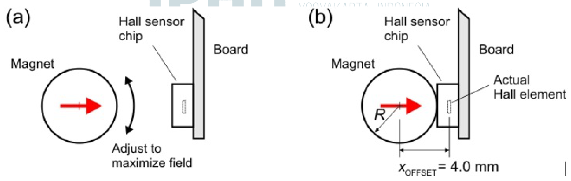
The -axis is along the magnetization axis of the diametric magnet as shown in Figure 6a and refers to the distance from the center of diametric magnet to hall probe sensor inside the sensor chip. Please refer to issue of offset shown in Figure 6b.
We will perform measurements only in the "Near field" region:
A.1 Record zero offset () of the Teslameter without any magnet nearby. Subtract subsequent field measurement with this value. [0,1 т.]
A.2 Measure magnetic field vs. in the near field region ! Where is the position measured from the center of the magnet. Record and plot your result on the answer sheet. Follow the "HINT & DIRECTIONS" below. [1,15 т.]
A.3 Use your experimental data to determine the value of the exponent . [0,75 т.]
A.4 Determine the magnet's magnetization . [0,5 т.]
HINTS & DIRECTIONS:
- Turn off the Tesla meter if not in use to save battery!
- For Teslameter, wait approximately ~2 sec for each data point before taking reading.
- Note that is measured from the center of magnet. Magnet radius is mm.
- Use recommended measurement setup in Fig. 5c.
- See Fig. 6a, adjust the rotation of the magnet so its magnetization is pointing to the Hall sensor thus maximizing the field. You can use the yellow round sticker to mark the magnetization direction on the magnet.
- When the Hall sensor touches the magnet the actual distance between the center of the magnet and the actual Hall sensor element is the offset value given as: mm
- Start your measurement with Hall sensor at mm! Don't use the data when the sensor touches the magnet ( mm) as the sensor is saturated or the probe is flexing during touch.
[2] The Magnetic Levitation effect and Magnetic Susceptibility () (1 pt.)
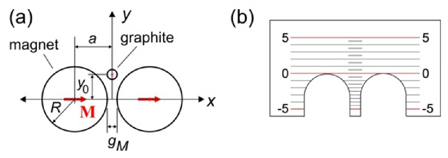
The PDL trap also demonstrates magnetic levitation effect. The graphite levitates at the center of the trap at height as shown in Fig. 7(a). The graphite is repelled by the magnet with a force that depends on the magnetic susceptibility and the rod position . Magnetic susceptibility describes how much a material gets magnetized in response to an applied field. It appears in relation: where is the magnetic permeability of the material. This magnetic repulsion force on a graphite rod in the PDL trap is given as:
Note that when is positive the force is directed upwards and there is a negative sign in the formula. Here is the volume of the graphite rod, is the volume magnetization of the magnet (obtained from Question 1), is the position of the magnet center given as: (see Fig. 7a) where is the gap between magnets: mm. is the dimensionless function for the magnetic repulsion force in this trap given as:
A.5 Place gently a graphite rod HB/0.5 and length = 8 mm. Measure the levitation height of the rod (see Fig. 7a)! Hint: Use the insert ruler provided as shown in Fig. 7b. Press the ruler on the magnets to read the position of the graphite rod. [0,1 т.]
A.6 Use the result from part A.5 to determine the magnetic susceptibility of the graphite rod. [0,8 т.]
A.7 What kind of magnetic material is graphite? Choose one: (i) Ferromagnetic; (ii) Paramagnetic; or (iii) Diamagnetic? [0,1 т.]
[3] The camelback potential oscillation and magnetic susceptibility () (1 pts)
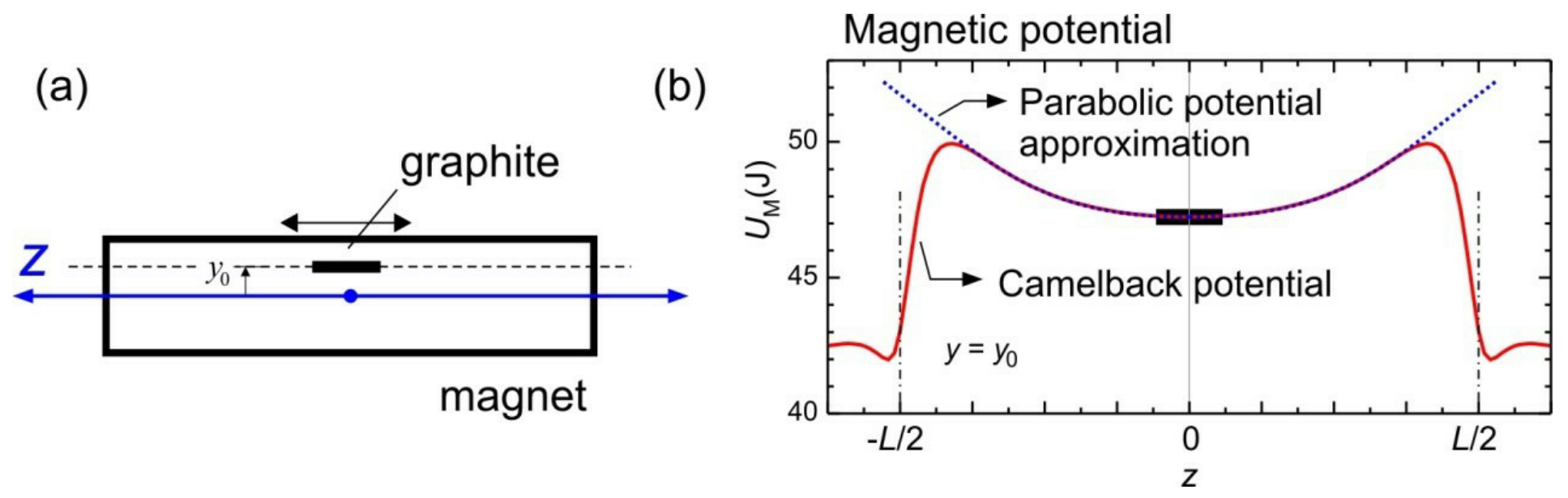
We will determine independently using the oscillation in the magnetic "camelback potential" of the PDL trap as shown in Fig. 8. For small amplitude ( mm) the magnetic potential can be approximated as a parabolic (shown as dotted curve in Fig. 8b):
where is the spring constant of the potential and is center of mass displacement of the rod. This spring constant depends on the magnet magnetization (from Question 1) and :
where is the magnetic permeability, is the volume of the graphite rod, is a constant for this magnetic trap setup.
Drop the graphite rod at the center of the magnetic trap. Adjust the platform level with the screw knobs so that the rod stays at the center of the trap. Displace the rod with a toothpick to induce oscillation along the camelback potential.
A.8 Perform an oscillation for the "HB/0.5" graphite and mm. Limit to small oscillation amplitude i.e. mm. Determine the oscillation period. (The oscillation will decay over time due to damping, ignore this damping effect). [0,2 т.]
A.9 Calculate the magnetic susceptibility () of the graphite using this oscillation. [0,8 т.]
[4] Oscillator quality factor () and estimate of air viscosity (3 pt.)
We observe that the graphite rod oscillation is damped due to the air friction and we want to understand how the friction depends on the size of the graphite rod (diameter and length) and estimate the air viscosity . The motion of the rod can be modeled as underdamped oscillation: as shown in Fig. 3(a) where is the initial amplitude and is the angular frequency and is time. The amplitude decays with time by a factor of where is the damping time constant. This determines the oscillator "quality factor" defined as: . If the oscillation is underdamped, is critically damped and is overdamped. This quality factor is important for designing PDL trap as seismometer or tiltmeter sensors.
We can calculate the damping time constant by approximating the cylinder rods as long ellipsoid and calculate the Stokes drag force. The damping time constant is given as:
where , and are the mass density, radius and length of the graphite rod and is the viscosity of the air. We want to estimate the air viscosity using this model.
A.10 We need to determine the damping time constant of the oscillation . Sketch how you measure in a simple way. [0,5 т.]
A.11 Perform oscillation damping experiments with a group of rods with various diameters and fixed length of 8 mm. Determine the damping time constant for each rods. [1,5 т.]
A.12 Determine the air viscosity . [1 т.]
[5] PDL Trap Seismometer (0.5 pt.)
SECTION B. SENSOR APPLICATIONS
Imagine you are designing seismometer using this PDL magnetic trap. For seismometer application we want very high sensitivity or very low acceleration "noise floor" i.e. the lowest acceleration that it can detect. This acceleration noise floor is given as (in unit of ):
where is the Boltzmann constant, is the temperature (see Constants and Data), and is the mass of the rod, all are in SI units. In Question 4 you have measured of several graphite diameters. Pick one that you think will serve as the best seismometer.
B.1 Which diameter of rod do you choose? [0,2 т.]
B.2 Calculate the seismometer acceleration noise floor () for the rod of your choice. [0,3 т.]
[6] PDL Trap Tiltmeter (2 pt.)
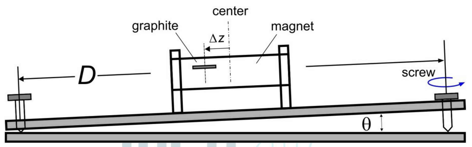
We will investigate the PDL trap as a very sensitive tiltmeter to monitor volcano. The change in the ground inclination is simulated by turning the screw and we want to determine the screw thread size where is the change of height per unit turn. We show that by measuring displacement of the graphite rod in the trap we can measure the inclination (tilt) precisely.
Use pencil rod HB/0.5 and length mm in this experiment. Start from the center position. Assume the camelback potential can be approximated as harmonic potential like in problem 3:
B.3 Derive the relation theoretically between displacement with the screw thread size and the number of turns . [0,5 т.]
B.4 By turning the screw slowly, determine the rod displacement vs. the number of screw turns . Determine the thread size . [1,25 т.]
B.5 When the ground tilt changes we want the graphite rod to go to equilibrium as fast as possible (instead of sustaining very long oscillation) to allow easy reading. What is the ideal factor for a tiltmeter? [0,25 т.]
AE2 — Parallel Dipole Line Magnetic Trap for Earthquake & Volcanic Sensing (10 points)
| Student Code | ||||||
|---|---|---|---|---|---|---|
A. BASIC CHARACTERISTICS OF PDL TRAP
1. Determination of the magnet's magnetization () (2.5 pt.)
Question — Answer — Marks
A.1 — 0.1 pt.
Record zero offset () of the Teslameter without any magnet nearby. Subtract subsequent field measurement with this value.
A.2 — 1.15 pt.
Measure magnetic field vs. in the near field region ! Where is the position measured from the center of the magnet. Record and plot your result on the answer sheet.

A.3 — 0.75 pt.
Use your experimental data to determine the value of the exponent .
A.4 — 0.5 pt.
Determine the magnet's magnetization .
2. The Magnetic Levitation effect and Magnetic Susceptibility () (1.0 pt.)
Question — Answer — Marks
A.5 — 0.1 pt.
Place gently a graphite rod HB/0.5 and length = 8 mm in the trap. Measure the levitation height of the rod (see Fig. 7a)! Hint: Use the insert ruler provided as shown in Fig. 7b. Press the ruler on the magnets to read the position of the graphite rod.
A.6 — 0.8 pt.
Use the result from part A.5 to determine the magnetic susceptibility of the graphite rod.
A.7 — 0.1 pt.
What kind of magnetic material is graphite? Choose one: (i) Ferromagnetic; (ii) Paramagnetic; or (iii) Diamagnetic?
3. The camelback potential oscillation and magnetic susceptibility ()
Question — Answer — Marks
A.8 — 0.2 pt.
Perform an oscillation for the "HB/0.5" graphite and mm. Limit to small oscillation amplitude i.e. mm. Determine the oscillation period. (The oscillation will decay over time due to damping, ignore this damping effect).
A.9 — 0.8 pt.
Calculate the magnetic susceptibility () of the graphite using this oscillation.
4. Oscillator quality factor () and estimate of air viscosity (4.0 points)
Question — Answer — Marks
A.10 — 0.5 pt.
We need to determine the damping time constant of the oscillation . Sketch how you measure in a simple way!
A.11 — 1.5 pt.
Perform oscillation damping experiments with a group of rods with various diameters and fixed length of 8 mm. Determine the damping time constant for each rods
A.12 — 1 pt.
Determine the air viscosity .
B. SENSOR APPLICATION OF THE PDL TRAP
5. PDL Trap Seismometer (0.5 pt.)
Question — Answer — Marks
B.1 — 0.2 pt.
Which diameter of rod do you choose?
B.2 — 0.3 pt.
Calculate the seismometer acceleration noise floor () for the rod of your choice.
6. PDL Trap Tiltmeter (2 pt.)
Question — Answer — Marks
B.3 — 0.5 pt.
Derive the relation theoretically between displacement with the screw thread size and the number of turns .
B.4 — 1.25 pt.
By turning the screw slowly, determine the rod displacement vs. the number of screw turns . Determine the thread size .
B.5 — 0.25 pt.
When the ground tilt changes we want the graphite rod to go to equilibrium as fast as possible (instead of sustaining very long oscillation) to allow easy reading. What is the ideal factor for a tiltmeter?
Отговори
The official sample key gives M = 1.1×10⁶ A/m for subsequent questions; graphite is diamagnetic, χ ≈ −1.85×10⁻⁴ by levitation and −1.5×10⁻⁴ by oscillation; μA = 38.6×10⁻⁶ Pa.s; choose HB/0.9 for an = 1.5×10⁻⁸ m/(s² Hz⁰·⁵); S = 0.75 mm/turn and ideal tiltmeter Q = 0.5.
These are the printed official sample results; individual measured data may differ. The official A.9 algebra lacks a minus sign in its second expression, and B.4 prints 22.8 < D < 22.2 cm.
Решение
E2. Marking Scheme & Solution
Parallel Dipole Line Magnetic Trap for Earthquake & Volcanic Sensing (10 points)
1. Determination of the magnet's magnetization () (2.5 pts)
A. BASIC CHARACTERISTICS OF PDL TRAP
A.1 Record zero offset () of the Teslameter without any magnet nearby. Subtract subsequent field measurement with this value
Example from a Teslameter unit: mT
Marks
0.08 pts range (-10 mT to 10 mT)
Correct unit: 0.02 pts [0,1 т.]
A.2 Measure magnetic field vs. in the near field region . Where is the position measured from the center of the magnet. Record and plot your result on the answer sheet.
mm, mT. is measured from surface.
| (mm) | (mm) | (T) | (T) | in m | in T |
|---|---|---|---|---|---|
| 3 | 7 | 0.1576 | 0.1567 | -4.962 | -1.853 |
| 4 | 8 | 0.1186 | 0.1177 | -4.828 | -2.139 |
| 5 | 9 | 0.0951 | 0.0942 | -4.710 | -2.362 |
| 6 | 10 | 0.0785 | 0.0776 | -4.605 | -2.556 |
| 7 | 11 | 0.0657 | 0.0648 | -4.510 | -2.736 |
| 8 | 12 | 0.0579 | 0.0570 | -4.423 | -2.864 |
| 9 | 13 | 0.0445 | 0.0436 | -4.343 | -3.132 |
| 10 | 14 | 0.0371 | 0.0362 | -4.269 | -3.318 |
| 12 | 16 | 0.0321 | 0.0312 | -4.135 | -3.466 |
Plot:
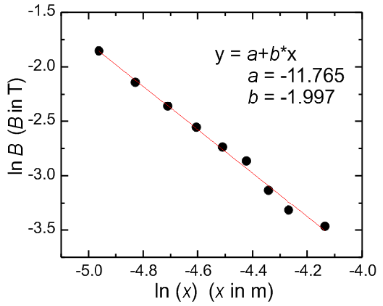
Marks
Correct label and unit for data: 0.1 pts
Number of correct data for mm: 0.05 pts for each correct data, max 0.45 pts
Plot:
- Correct axis label and unit: 0.05 pts
- Using around 75% of plot area: 0.05 pts
- For each correct data point: 0.05 pts, max. 0.4 pts
- Adding trendline: 0.1 pts [1,15 т.]
A.3 Use your experimental data to determine the value of the exponent .
Linear regression (LR) :
LR yields: and
The power exponent:
Note that this is in very good agreement with the exact result: at short distance a diametric (or a dipole line) magnet has dependence. See Ref. [1], Fig. 2c.
Marks
Obtaining from graph: 0.05 pts
Obtaining from linear regression: 0.1 pts
Result:
: 0.65 pts
: 0.35 pts
Result with wrong sign:
: 0.4pts
: 0.1pts
More than two sig. figs.: minus 0.05 pts [0,75 т.]
A.4 Determine the magnet's magnetization .
This is close to the more accurate results from more extensive measurements to far field (see Ref. [1], Fig. 2c) and we use this value for subsequent questions:
Marks
Correct unit: 0.05 pts
Obtaining intercept from graph: 0.025 pts
Obtaining intercept from LR: 0.05 pts
Correct formula for and/or : 0.1 pts
Result for (x10⁶ A/m):
0.9 - 1.4: 0.3 pts
0.1 - 2.5: 0.15 pts
More than 2 sig. figs.: minus 0.05 pts [0,5 т.]
2. The Magnetic Levitation Effect and Magnetic Susceptibility () (1 pts)
A.5 Place gently a graphite rod HB/0.5 and length = 8 mm. Measure the levitation height of the rod (see Fig. 7a). Hint: Use the insert ruler provided as shown in Fig. 7b. Press the ruler on the magnets to read the position of the graphite rod
We levitate graphite HB/0.5, mm. Using the insert-ruler, we measure approximately mm from the top of the magnet surface. Thus: mm mm
Marks
correct unit: 0.02
mm: 0.08 pts
partial credit: Only mm: 0.03 pts [0,1 т.]
A.6 Use the result from part A.5 to determine the magnetic susceptibility of the graphite rod.
Solving for :
We calculate: mm mm.
Using mm: ,
Using the correct A/m; and mm, kg/m³ we have: .
Note that this is very good agreement with the literature value for graphite pencil lead: (see Ref.[1], pg. 2 & Ref.[2]). The sign is negative indicating a diamagnetic material.
Marks
Correct expression for : 0.4 pts
Result for (x10⁻⁴)
-(1.4 to 2.6): 0.4 pts
-(0.5 to 4): 0.2 pts
Wrong sign: minus 0.1 pts [0,8 т.]
A.7 What kind of magnetic material is graphite? Choose one: (i) Ferromagnetic; (ii) Paramagnetic; or (iii) Diamagnetic?
(iii) Diamagnetic. Because:
(1) Graphite is repelled by magnetic field
(2) The sign of is negative.
Marks
Correct choice: 0.1 pts [0,1 т.]
3. The camelback potential oscillation and magnetic susceptibility () (1 points)
A.8 Perform an oscillation for the "HB/0.5" graphite and mm. Limit to small oscillation amplitude i.e. mm. Determine the oscillation period. (The oscillation will decay over time due to damping, ignore this damping effect).
Example, we measured 5 oscillations of HB/0.5 with length mm. We displaced it by ~3 mm and let it oscillates. We measured 5 oscillation periods:
| Trial | (s) |
|---|---|
| 1 | 6.12 |
| 2 | 6.13 |
| 3 | 6.14 |
Average: s
Marks
Correct label and unit: 0.02 pts
Number of correct data each 0.01 pts, max 0.03 pts
Number of oscillation
: 0 pts
: 0.05 pts
s: 0.1 pts [0,2 т.]
A.9 Calculate the magnetic susceptibility () of the graphite using this oscillation
For harmonic oscillator: , solving for :
Using the correct A/m.
Using , and s, we obtain .
Note that this is in good agreement with the literature value of the graphite pencil lead: (Ref.[1], pg. 2); and the sign is negative indicating a diamagnetic material.
Marks
Correct expression for : 0.4 pts
Result for (x10⁻⁴)
-(1.4 to 2.6): 0.4 pts
-(0.5 to 4): 0.2 pts
Wrong sign: minus 0.1 pts [0,8 т.]
4. Oscillator quality factor () and estimate of air viscosity (3.0 points)
A.10 We need to determine the damping time constant of the oscillation . Sketch how you measure in a simple way.
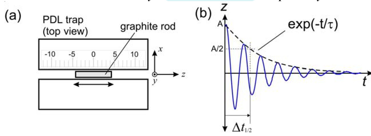
The trick is to use "half-time" concept of exponential decay. We set the oscillation and measure the time taken for the amplitude to halve. The lifetime is:
Marks
Correct idea: 0.3 pts
Correct expression for : 0.2 pts [0,5 т.]
A.11 Perform oscillation damping experiments with a group of rods with various diameters and fixed length of 8 mm. Determine the damping time constant for each rods
We displaced the graphite by ~4 mm, started the stopwatch and then waited until it decays to half.
| Trial | Diam. (mm) | Actual Radius (mm) | (s) | Mean (s) | (s) | (mm²) |
|---|---|---|---|---|---|---|
| 1 | 0.3 | 0.19 | 3.89 | 3.913 | 5.646 | 0.117 |
| 3.97 | ||||||
| 3.88 | ||||||
| 2 | 0.5 | 0.28 | 7.69 | 7.617 | 10.989 | 0.224 |
| 7.57 | ||||||
| 7.59 | ||||||
| 3 | 0.7 | 0.35 | 8.77 | 8.82 | 12.73 | 0.322 |
| 8.81 | ||||||
| 8.88 | ||||||
| 4 | 0.9 | 0.45 | 12.4 | 11.70 | 16.88 | 0.482 |
| 11.33 | ||||||
| 11.38 |
Marks
Correct label and unit 0.1
Number of correct data for each diameter (4):
: 0.1 pts
: 0.25 pts
(max 1.0 pts)
Positive monotonic trend for vs. diameter from 0.3 to 0.9 mm with to 20 sec: 0.4 pts [1,5 т.]
A.12 Determine the air viscosity
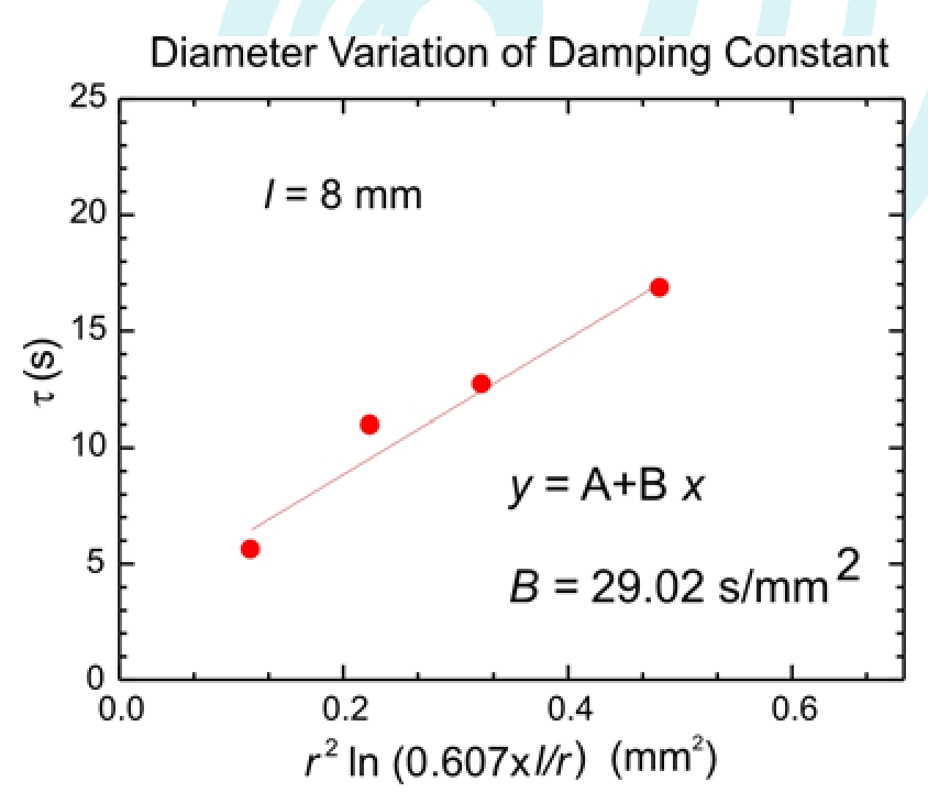
We have: , where: . We performed linear regression , with and . We obtain: s/mm².
Note that this is about 2.1x the actual viscosity of air of 18.2µ.Pa.s. The discrepancy is due to the ellipsoidal approximation of the Stokes drag (vs. the actual cylindrical shape of the rod) and the proximity effect of the rod to the magnet (wall effect). Another factor is the crude nature of our manual determination. See Ref. [1], pg. 8.
Marks
Correct unit: 0.05
Obtaining result with linear regression or plot: 0.25 pts
Result (x10⁻⁶ Pa.s):
20 - 60: 0.7 pts
10 - 80: 0.4 pts
1 - 100: 0.1 pts [1 т.]
5. PDL Trap Seismometer (0.5 pts)
B. SENSOR APPLICATION OF THE PDL TRAP
B.1 Which diameter of rod do you choose?
To obtain the lowest acceleration noise floor "an" we should choose the largest diameter graphite i.e. 0.9 mm, because their damping time is the longest and the mass is the largest.
Marks
Correct answer: 0.2 pts [0,2 т.]
B.2 Calculate the seismometer acceleration noise floor () for the rod of your choice!
For HB/0.9 and length mm:
We use s; and K, we have: kg:
Marks
Correct unit: 0.1
Correct answer: 0.2 pts [0,3 т.]
6. PDL Trap Tiltmeter (2 pts)
B.3 Derive the relation theoretically between displacement with the screw thread size and the number of turns .
From Question 3, we also have :
Marks
Correct expression: 0.5 pts
Partial credit
: 0.2 [0,5 т.]
B.4 By turning the screw slowly, determine the rod displacement vs. the number of screw turns . Determine the thread size
We measured the distance between screws: cm, and we used the period from Q3: s
| (mm) | (turn) | |
|---|---|---|
| 0 | 0 | 0 |
| 0.5 | 135 | 0.375 |
| 1 | 270 | 0.75 |
| 1.5 | 450 | 1.25 |
| 2 | 585 | 1.625 |
| 2.5 | 720 | 2.0 |
| 3 | 855 | 2.375 |
| 3.5 | 945 | 2.625 |
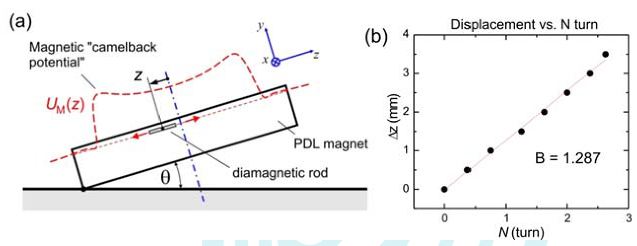
By performing linear regression:
We have mm/turns: mm/turn.
This is reasonably close to the actual value of the thread size: mm/turn.
Marks
Correct label and unit: 0.1 pts
Distance between screws:
cm: 0.1 pts
Number of correct data:
sets: 0 pts
3-5 sets: 0.15 pts
sets: 0.25 pts
Obtaining result with linear regression or plot: 0.2 pts
Result:
: 0.55 pts
: 0.15 pts
Correct unit for : 0.05 [1,25 т.]
B.5 When the ground tilt changes we want the graphite rod to go to equilibrium as fast as possible (instead of sustaining very long oscillation) to allow easy reading. What is the ideal factor for a tiltmeter?
We need critical damping thus:
Marks
Correct : 0.25 pts [0,25 т.]
REFERENCES:
[1] Gunawan, O. & Virgus, Y. The one-dimensional camelback potential in the parallel dipole line trap: Stability conditions and finite size effect. J. Appl. Phys. 121, 133902, (2017). DOI:10.1063/1.4978876.
[2] Gunawan, O., Virgus, Y. & Fai Tai, K. A parallel dipole line system. Appl. Phys. Lett. 106, 062407, (2015). DOI: 10.1063/1.4907931.
Теми и трудност
Оценена трудност: 4/5.
Магнетизъм и индукция · Механика · Флуиди · Магнитно поле · Механични трептения · Вискозитет и съпротивление
Предпоставки: Гимназиална подготовка, Разширена олимпиадна подготовка
Оригинал в Архива: exp2.pdf · официални решения: exp2_sol.pdf · допълнителни данни: exp2_anssheet.pdf · допълнителни данни: exp_instructions.pdf