IPhO 2018, Експеримент — Задача 1. Paper transistor
Paper transistor (10 points) · 23 юли 2018 г. · 10 т.
Внимание: Бележка към темата
One complete connected Paper transistor experiment with Parts A–D and 20 native requests: 13 question, 19 official key and 15 native answer-sheet pages. The key version v1.4 is dated July 23, 2018. Complete apparatus, numeric sample measurements, derivations, graphs and blank forms retained. Printed source discrepancies remain with attributed local notes. No overall time limit, separate residual-current value or missing time measurements are invented.
Official key edition
Solutions to Experimental Problem 1 — Paper transistor. Authors: Elvira Fortunato, Luís Pereira, Rui Igreja, Paul Grey, Inês Cunha, Diana Gaspar, Rodrigo Martins. July 23, 2018, v1.4. The obtained historical key carries a “Confidential” watermark.
Условие
Electronic technology in modern society is based on a simple, yet powerful device: the transistor, which can be used both as a switch and as an amplifier. The switch mode is used for storage and processing of digital information.
Here we will analyse two types of Field Effect Transistors (FET): JFET (Junction Field Effect Transistor) and the TFT (Thin Film Transistor).
We shall briefly explain here how a FET works. A FET is a non-linear 3 terminal device (the terminals being named Gate: G; Source: S; and Drain: D) that can control the current flow between Source and Drain by acting upon the voltage applied between the Gate and the Source. In a simple, although imperfect analogy, a FET works similarly to a water tap, the knob acting as the Gate controlling the water flow.
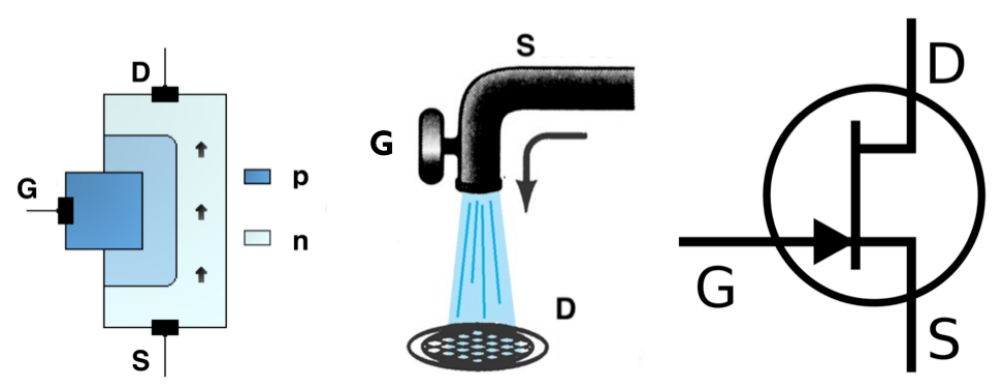
The Junction-FET (JFET) relies upon the properties of the junction between two types of a semiconducting material, such as p and n doped silicon, hence its name. A JFET has a narrow channel through which the current flows between Source and Drain, and in a n-channel FET this channel is made of n-type material. The width of such channel can be controlled in a precise way by applying a negative voltage between the Gate and the Source, . For a fixed , the current flowing between Source and Drain depends non-linearly on the applied voltage between Drain and Source, . For small voltages, however, the current does depend linearly on the applied voltage, thus the JFET displays ohmic behaviour. The output resistance, , however, does depend strongly on the applied voltage, closely following the law:
where is the output resistance at and is a JFET parameter called the pinch-off voltage. Clearly, at the pinch-off voltage, the FET blocks current flow.
For any fixed , the current between Source and Drain will start to depart from the linear behaviour as we increase , and will at some point saturate at an almost constant value. Let be the saturation current when . In the saturation regime (large applied ), the saturation current will depend on in the following way:
We should stress two very important characteristics of a JFET. Although its voltage controlled output resistance can be quite low, the input resistance () is extremely high, typically larger than , so this device uses very little input current. Also, the capacitance of a small JFET is quite low making it a very fast device than can 'open and close' beyond MHz rates.
We now proceed to describe how a different type of FET, the TFT, works.
As any other FET, the TFT permits the control of a current between two contacts, the Drain and Source electrodes, by means of an applied potential at the third electrode, the Gate.
The Gate electrode is physically separated from the semiconductor layer by a dielectric that allows for the establishment of a vertical electrical field that will control the free charge carriers existing in the semiconductor (field effect). The dielectric layer can be replaced by an electrolytic membrane such as paper where mobile ions exist (see Figure 2) and in this case the voltage applied at the Gate will push ions with opposite charge to the semiconductor interface, creating a sheet of ionic charges that will modulate the free carriers' density existing within the semiconductor (Electrolyte Gated Transistors - EGTs). Researchers at Universidade Nova, Lisbon, were pioneers in developing in 2008 the "paper transistor", and are world leaders in this field.
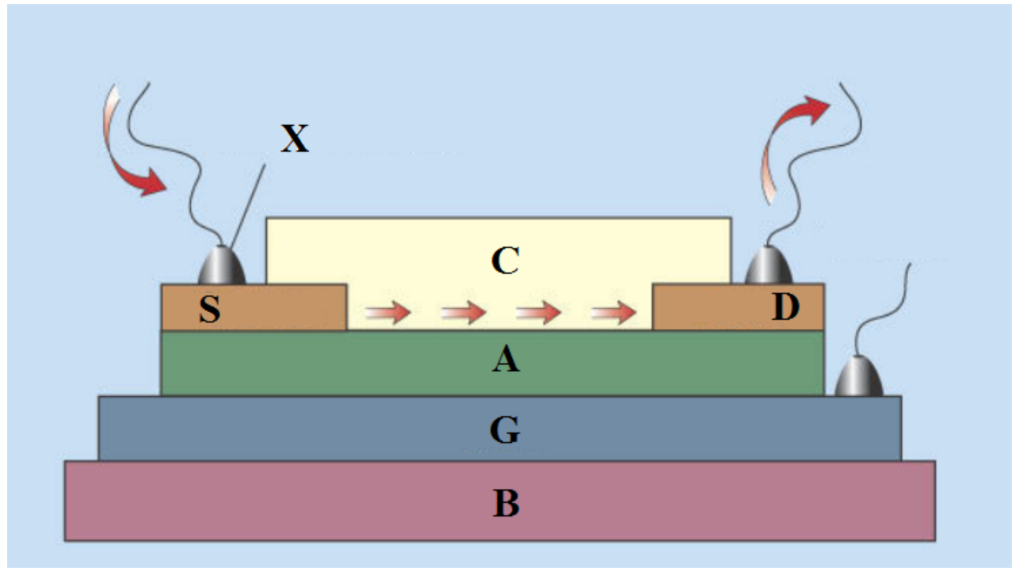
Similarly to JFETs, TFT transistors can operate in two fundamental operation modes, a linear mode and a saturation mode. In contrast to JFET, TFT intrinsic capacitance is a relevant parameter for the device performance.
In this experimental problem you will examine how an n-channel JFET and a paper TFT work.
You will determine the Characteristic Curves (CCs) of these devices by measuring the current between S and D () through the application of distinct voltages at G () and D ().
The two most important CCs are the output and the transfer curves:
- Output Curve: For this curve the current between Source and Drain () will be measured and plotted as a function of the voltage between Source and Drain (), with swept from up to , in steps, while keeping constant.
- Transfer Curve: For this curve will be measured and plotted against . will be kept constant at a suitable value for the transistor to work in the saturation mode and will be swept in steps from to .
Equipment
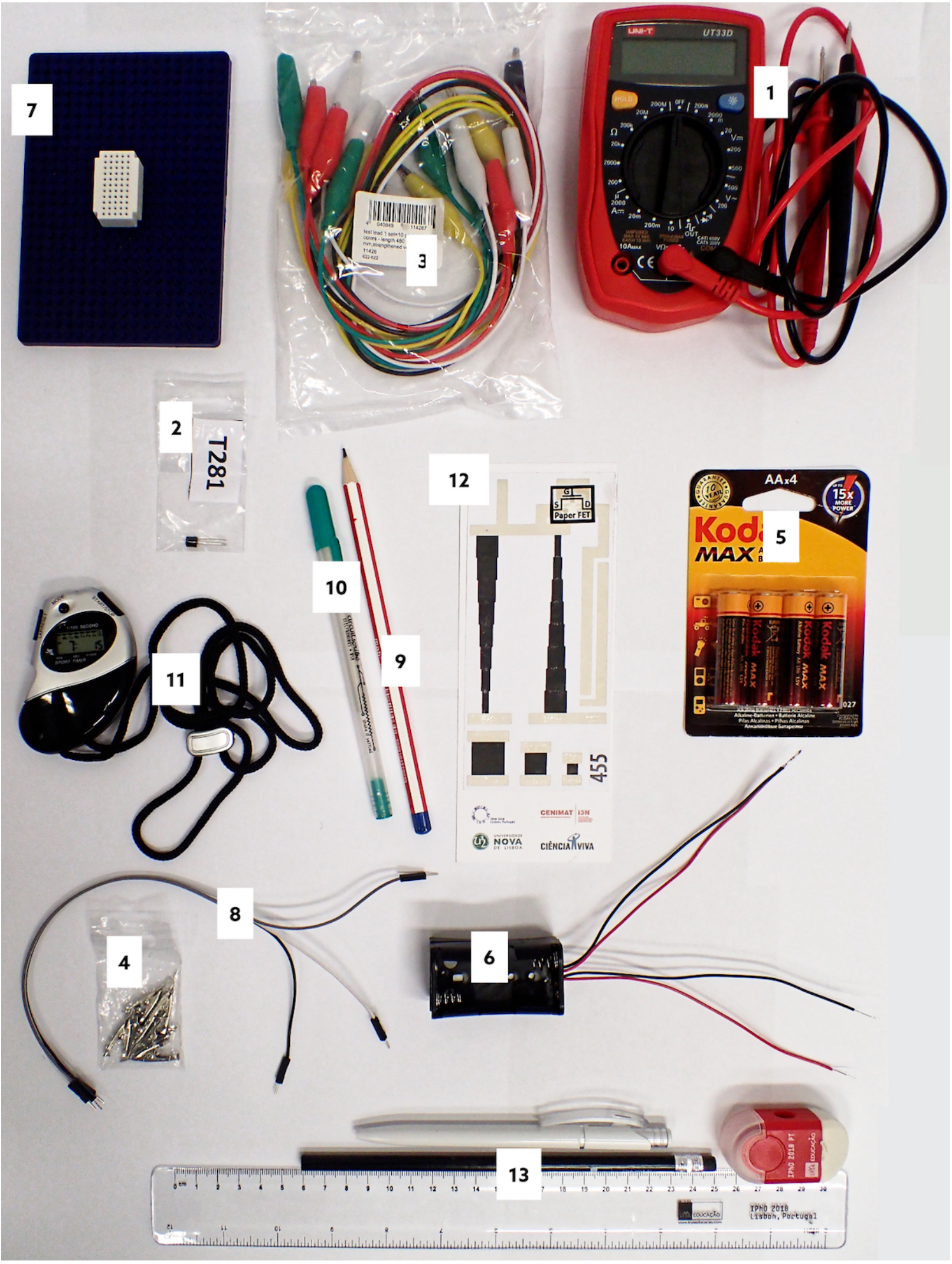
The following set of equipment (Figure 3) is provided for this experimental problem:
- multimeter
- JFET transistor (provided inside a labelled plastic bag)
- cables (10) with alligator clips
- flat alligator clips (4, provided inside a plastic bag)
- battery pack ()
- battery holder
- mini-breadboard with support
- jumper wires (3) to connect to the mini-breadboard
- HB pencil
- silver ink conductive pen (Circuit Scribe)
- chronometer
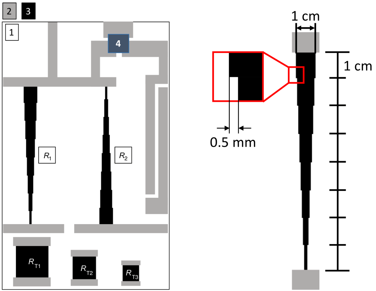
- sheet of paper with printed circuits and an embedded TFT that uses paper as dielectric layer (Figure 4)
- bag with writing material (1 pen, 1 pencil, 1 eraser/sharpener, 1 ruler)
Important precaution:
Do not fold the sheet of paper with the printed circuits and embedded transistor as this will easily damage it. Try to leave it as flat as possible during measurements in order to reach best results.
For the measurements it is important to take into account the following important information:
- The multimeter should always be operated in DC mode.
- The multimeter does not autorange and you should carefully choose the most appropriate ranges for your measurements. In case a overflow occurs the display will show either "1" or "-1" (left justified on the display), for positive and negative values, respectively, and you should change to a lower range.
- The low-current ranges are protected by a fuse. Avoid by all means to create a short circuit between the battery and the multimeter because a high current will blow up the fuse!
- The internal resistance of the multimeter when operating in voltmeter mode is .
- When operating as ammeter, the internal resistance of the multimeter depends on the range as shown in the following table:
| Range | |
|---|---|
| 1.0 | |
| 10 | |
| 100 |
Table 1. Internal resistance of the provided multimeter when operated as ammeter.
Thus, when the multimeter is being used in DC ammeter mode, there will be a voltage drop up to between its terminals at full scale when operated in any of the 3 available DC ranges.
Source note: The original overflow instruction says “change to a lower range”; that printed instruction is retained.
Part A. Circuit dimensioning (2.5 points)
To achieve the necessary and voltages you will use two carbon resistors printed on paper ( and , see Fig. 4) and voltage divider circuitry to dimension the circuit for the right potential drops. and will be the total resistance () of a voltage divider circuit. When applying a constant voltage (in this case about from the battery) across , for instance, we will see a voltage drop along it from (, the positive contact of the battery) to ground (; from now on, we designate as ground the common contact of the two battery packs). can be divided into essentially two resistances ( and ) to achieve the desirable (Figure 5).
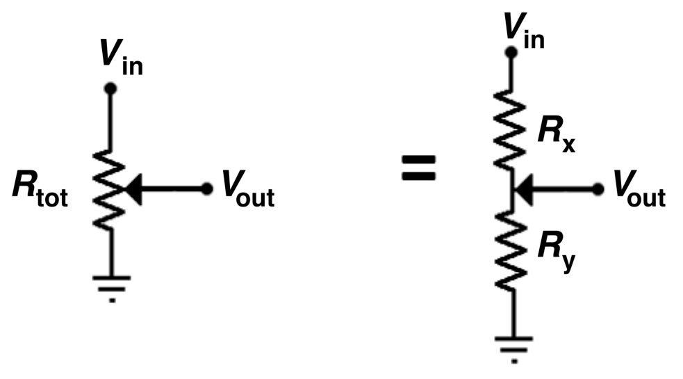
A.1 Write down the expression for the output voltage, , as a function of and resistances and . [0,2 т.]
A.2 Measure the resistance of the three test resistors on the bottom part of the sheet (, and ) with the multimeter. Carry out enough measurements with different positions on the silver contacts. Enter the values in the Answer Sheet. Calculate the average value and estimate the uncertainty for the resistance of each test resistor. [0,5 т.]
A.3 Show that the resistance of a square thin film with a certain resistivity, , should be independent of the length of its side. This size-independent resistance is called sheet resistance and is denoted . [0,3 т.]
A.4 Calculate the average value of the sheet resistance of the carbon film from the data in A.2 and obtain the resistivity, , of the carbon film with an estimation of its uncertainty (consider a thickness of the carbon film of ). [0,4 т.]
A.5 Show that the theoretical value of the and resistances is , . Measure and and write down the values in the Answer Sheet. Determine the experimental value of and compare it with the theoretical value. [0,5 т.]
Using the provided silver ink pen, draw 7 equally spaced conductive lines along each of the provided resistors (as exemplified in Figure 6). These individual lines will serve as the contact points for the voltage dividers.
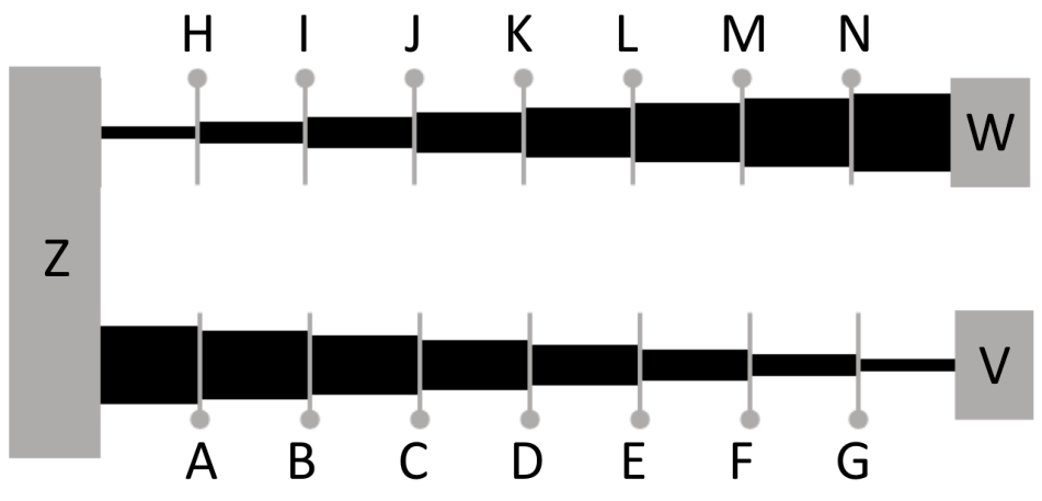
A.6 Measure the resistances and for all contact points. is defined as the resistance between the contact point and points V (resistor 1) or W (resistor 2), and is defined as the resistance between the contact point and point Z. Fill the provided tables in the Answer Sheet. [0,3 т.]
Insert the 4 AA batteries in the battery holder. Please observe carefully the correct battery polarity and make sure you do not produce a short circuit. Then, physically connect the battery pack as depicted in Figure 7. Make sure you do not damage the silver tracks with the alligator clips.
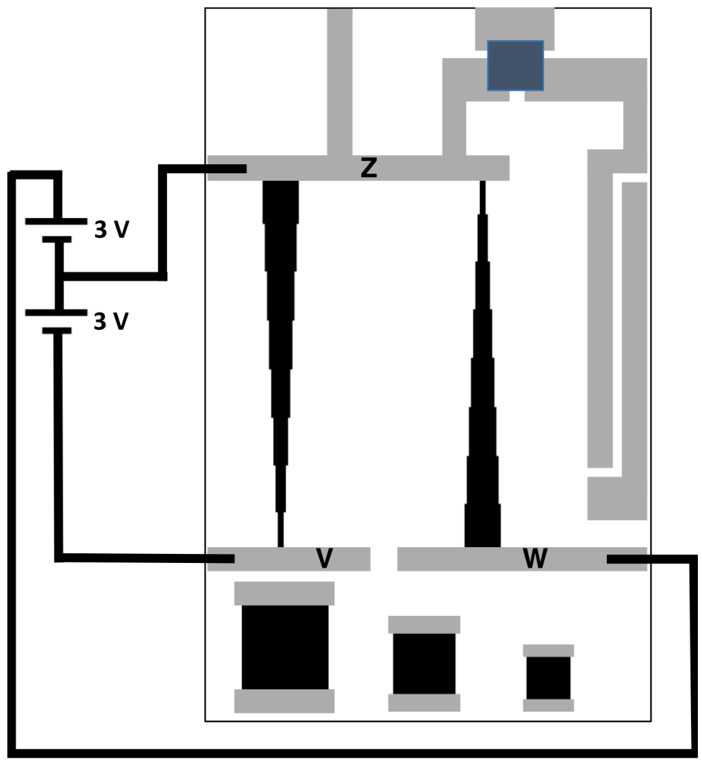
A.7 Measure at each contact point, being the voltage measured with respect to point Z and enter the values in the provided tables in the Answer Sheet. [0,3 т.]
This concludes the circuit dimensioning part and you can now proceed to measure the CCs of the JFET transistor.
Part B. Characteristic Curves of the commercial JFET transistor (4.5 points)
In order to characterise the JFET transistor you will use the setup depicted in Figure 8. Start by identifying the three contacts (S, D and G) on the provided JFET transistor - pay attention to the correct identification of the contacts, as the device is not symmetric! You may use the provided minibreadboard with support to mount the JFET transistor. The provided jumper wires are to be used with the mini-breadboard.
Using the provided cables, connect the Gate and the Source of the transistor to ground (point Z of the circuit, at ). Throughout this part of the problem, the Source of the JFET should always be kept connected to ground.
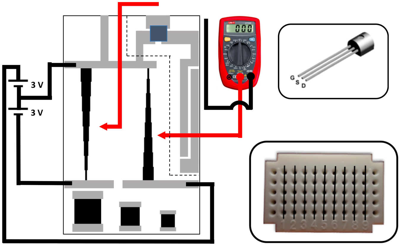
B.1 Connect the gate of the transistor to ground (). Then connect one of the cables of the multimeter, that should be used in DC current mode, to the drain of the transistor and with the other cable touch the point with the highest voltage available in the voltage dividers. Write down in the answer sheet the value of the current . [0,2 т.]
B.2 Measure the current for different positive voltages applied to the Drain, while keeping . Then change the circuit to apply a negative voltage between the Gate and the Source of the transistor () and repeat the measurements of as a function of the positive applied voltage between Drain and Source. Fill with your values the tables provided in the Answer Sheet. [0,8 т.]
When the voltage divider circuit is connected to a low resistance load (Figure 9), the voltage values provided by the voltage divider, , are different from the nominal values measured when the load is a high resistance, such as the case of a high impedance voltmeter.
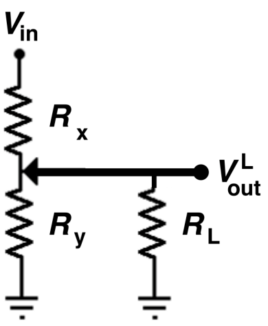
B.3 Consider that the voltage divider is connected to a load . Obtain an expression for the correction factor as a function of , and . [0,2 т.]
The JFET transistor has a low output resistance when , namely . However, this resistance increases significantly when the Gate is polarised negatively with respect to the Source. For the output resistance follows closely the law given by equation (1).
B.4 Using the appropriate correction factors, calculate , the voltage drop between Drain and Source, for all the points measured in B.2. Consider the following nominal data for the JFET used in this problem: , . [1,2 т.]
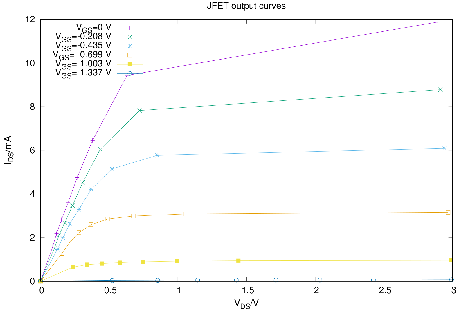
B.5 Plot the output curves for your JFET transistor. [0,5 т.]
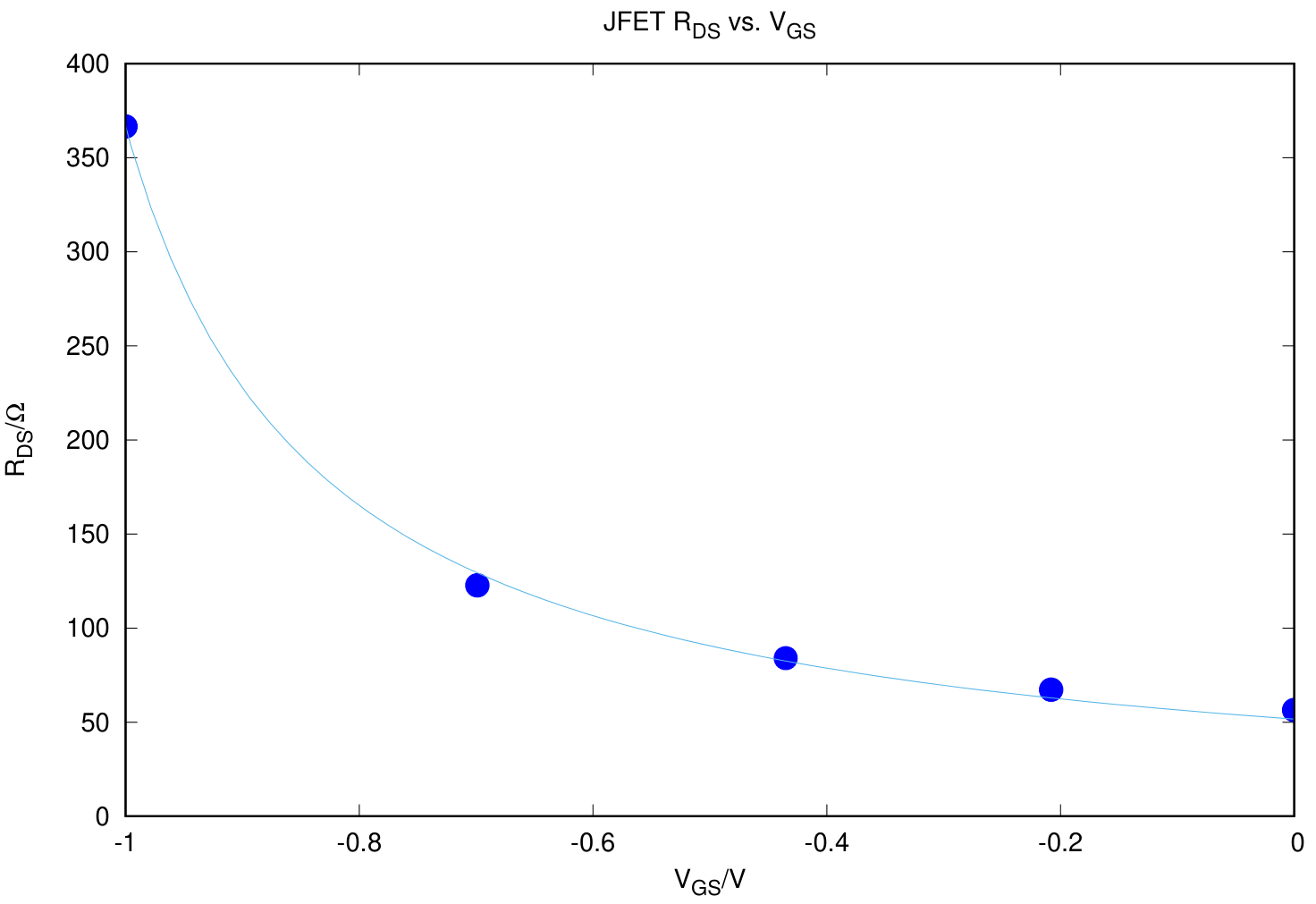
B.6 Consider the transistor in operation at small . Obtain the experimental values of of your JFET for different and plot the data. [0,5 т.]
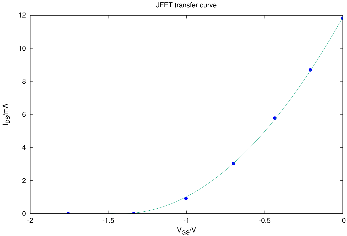
B.7 Plot the transfer curve of your JFET transistor for . [0,3 т.]
When the JFET transistor is in saturation mode, the current follows closely the law expressed by equation (2).
B.8 From the measured data, obtain and the pinch-off voltage, , for your device. Compare the value obtained of with the nominal value. [0,4 т.]
An important parameter of a JFET transistor, in particular when it is used in amplifiers, is the so called transistor transconductance, , defined as
For a function of two variables , the notation means the derivative of with respect to when is kept constant.
B.9 Obtain, from the measured transfer curve, the transconductance of your device for . Compare it with the calculated value obtained from the model equation (2). [0,4 т.]
Part C. The Paper Thin Film Transistor (2.0 points)
From now on, you discard the JFET, and all following tasks and questions relate to the paper thin film transistor (TFT) located in the upper corner of the printed circuit. The TFT Gate, Source and Drain are marked in Figure 10. Connect the TFT Gate and the Source to ground. Also in this part of the problem the Source of the paper TFT should always be connected to the common contact of the battery packs, i.e. , as shown in Figure 10. Polarise the transistor with , via one of the voltage circuit dividers (Figure 10). Check that a current is flowing through the ammeter.
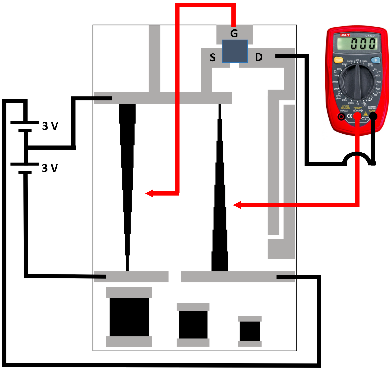
C.1 Apply . Close the transistor by applying . Wait for so that the the transistor closes. Write down in the answer sheet the residual value of the current, . Then open the transistor by putting , while keeping . Measure the current as function of time, starting at the instant when you open the transistor, for at least and collect the data in the answer sheet. [0,8 т.]
C.2 Plot . There is a superposition of two exponential processes in the time dependence, one with a much larger time constant () than the other (). Determine the shorter time constant, . [1,2 т.]
Part D. Inverter circuit (1.0 points)
In microelectronic circuitry one of the most important circuits is the inverter, that is able to invert a digital input. For instance if then and vice-versa. A transistor is once again at the basis of the circuit and one of the simplest designs is the so called common source amplifier, depicted in Figure 11, using a transistor and a load resistance (). In this case and is the voltage measured at the Drain electrode of the transistor. Thus, in this part we will monitor what happens to while sweeping from to .
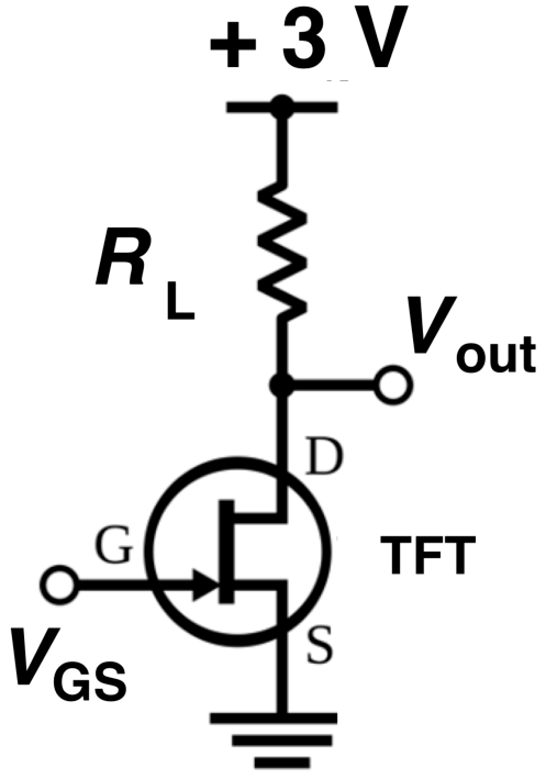
In the setup of Figure 11 the transistor is the paper TFT and is a load resistance you are going to add now, manually, by connecting the Drain contact of the transistor with the Vin contact using a pencil track, as indicated in Figure 12. While you write, you are actually depositing thin layers of conductive graphite on the paper so the more layers you draw on top of each other, the lower the resistance will get. While drawing make sure to continuously monitor its resistance. To pull Vout as close to as possible the load resistance should be large enough. So, while drawing the resistance, aim for a value close to the target value .
You can either use the pencil to decrease or the eraser to increase it. You should aim to obtain a value differing not more than 10% from the aimed value.
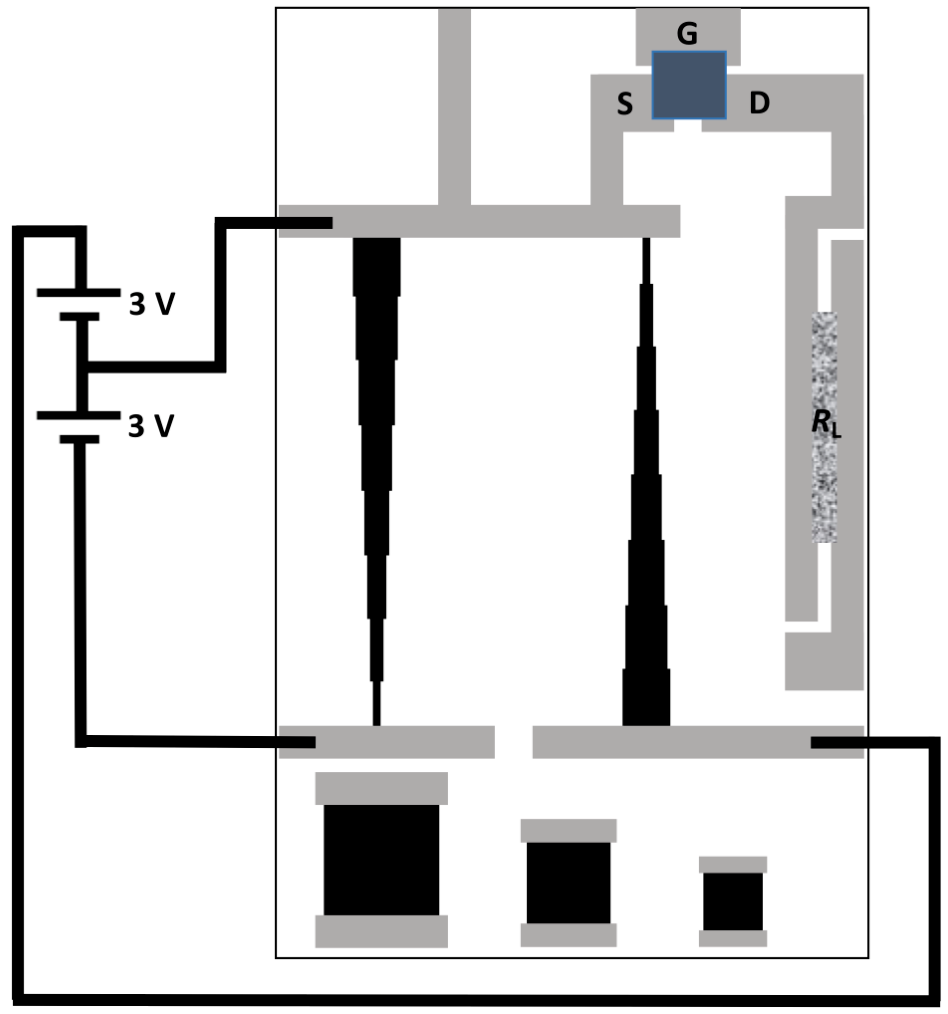
Use the included HB pencil and draw by hand a carbon resistor with value of to be used as a load resistor of the paper TFT to build the inverter circuit (see Figure 12).
D.1 Write down in the Answer Sheet the measured value you have reached. Setup the inverter circuit (Figure 12) using the carbon track resistor and the paper TFT. Before the measurement, remember that you should turn the transistor fully off by applying and wait for . Then measure as you sweep from to and take readings of with a stabilization time for each point up to a maximum of . Enter the measured values in the Answer Sheet. [0,5 т.]
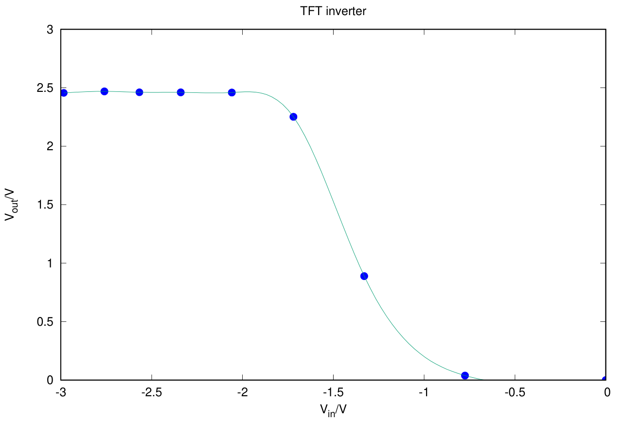
D.2 Plot the measured voltage transfer curve and draw a smooth trend curve through the data points. [0,5 т.]
Native answer sheets
These are the blank forms from the obtained 15-page official answer-sheet companion, in native page order. Blank cells and fields are deliberately left blank. They are not additional tasks or measured data.
Answer sheet A1-1
Write down the numbers 0 to 9 in the following table:
| 0 | 1 | 2 | 3 | 4 | 5 | 6 | 7 | 8 | 9 |
|---|---|---|---|---|---|---|---|---|---|
Part A: Circuit Dimensioning (2.5 points)
A.1 (0.2 pt)
A.2 (0.5 pt)
| # | |||
|---|---|---|---|
Answer sheet A1-2
A.3 (0.3 pt)
Demonstration:
A.4 (0.4 pt)
A.5 (0.5 pt)
Demonstration:
Measured values:
Answer sheet A1-3
A.6 (0.3 pt)
Resistor :
| Points | ||
|---|---|---|
| Z | ||
| A | ||
| B | ||
| C | ||
| D | ||
| E | ||
| F | ||
| G | ||
| V |
Resistor :
| Points | ||
|---|---|---|
| Z | ||
| H | ||
| I | ||
| J | ||
| K | ||
| L | ||
| M | ||
| N | ||
| W |
A.7 (0.3 pt)
| Points | Points | ||
|---|---|---|---|
| A | H | ||
| B | I | ||
| C | J | ||
| D | K | ||
| E | L | ||
| F | M | ||
| G | N | ||
| V | W |
Answer sheet A1-4
Part B: Characteristic Curves of the JFET transistor (4.5 points)
B.1 (0.2 pt)
B.2 (0.8 pt)
current values:
| Gate/Drain | Z | H | I | J | K | L | M | N | W |
|---|---|---|---|---|---|---|---|---|---|
| Z | |||||||||
| A | |||||||||
| B | |||||||||
| C | |||||||||
| D | |||||||||
| E | |||||||||
| F | |||||||||
| G | |||||||||
| V |
B.3 (0.2 pt)
Answer sheet A1-5
B.4 (1.2 pt)
Use the empty columns to enter corrections factors you deem necessary.
Gate A:
| Drain point | ||||||
|---|---|---|---|---|---|---|
Gate B:
| Drain point | ||||||
|---|---|---|---|---|---|---|
Answer sheet A1-6
B.4 cont.
Gate C:
| Drain point | ||||||
|---|---|---|---|---|---|---|
Gate D:
| Drain point | ||||||
|---|---|---|---|---|---|---|
Answer sheet A1-7
B.4 cont.
Gate E:
| Drain point | ||||||
|---|---|---|---|---|---|---|
Gate F:
| Drain points | ||||||
|---|---|---|---|---|---|---|
Answer sheet A1-8
B.4 cont.
Gate G:
| Drain points | ||||||
|---|---|---|---|---|---|---|
Gate V:
| Drain points | ||||||
|---|---|---|---|---|---|---|
Answer sheet A1-9
B.5 (0.5 pt)
Output curves:

Answer sheet A1-10
B.6 (0.5 pt)
Graph:

Answer sheet A1-11
B.7 (0.3 pt)
Transfer curve:

B.8 (0.4 pt)
B.9 (0.4 pt)
Measured transconductance:
Calculated transconductance from JFET model:
Answer sheet A1-12
Part C: The Paper Thin Film Transistor (2.0 points)
C.1 (0.8 pt)
Answer sheet A1-13
C.2 (1.2 pt)
Graph:

Auxiliary graph to determine :

Answer sheet A1-14
Part D: Inverter circuit (1.0 points)
D.1 (0.5 pt)
Answer sheet A1-15
D.2 (0.5 pt)
Graph:

Решение
Sketch of the solutions:
Part A. Circuit dimensioning (2.4 points)
Source note: The key heading prints 2.4 points. The question and answer-sheet headings print 2.5 points; both source values are retained.
A.1
Using Ohm’s law, the current through the voltage divisor is , and . Thus
A.1 (0.2 pt)
A.2 (0.5 pt)
Uncertainty in each measurement:
| # | |||
|---|---|---|---|
| 1 | 122.3 | 125.3 | 125.3 |
| 2 | 122.3 | 125.4 | 125.4 |
| 3 | 122.3 | 125.3 | 125.4 |
| 4 | 122.2 | 125.2 | 125.5 |
| 5 | 122.3 | 125.4 | 125.4 |
| 6 | 122.3 | 125.4 | 125.3 |
| 7 | 122.2 | 125.4 | 125.4 |
| 8 | 122.2 | 125.3 | 125.4 |
| 9 | 122.2 | 125.4 | 125.4 |
| 10 | 122.2 | 125.4 | 125.5 |
| 122.25 | 125.35 | 125.40 | |
| 0.05 | 0.07 | 0.07 |
A.3 (0.3 pt)
For a parallelepiped conductor of length , width and thickness , the resistance is given by
For a thin film of square shape, , thus
A.4
The weighted average value (weighed by ) of the sheet resistance is and .
A.4 (0.4 pt)
A.5 (0.5 pt)
For a rectangular thin film , thus
Measured values:
Comparison with the theoretical value: the average value is compatible, within the assigned error bar, with the theoretical value.
A.6 (0.3 pt)
Uncertainty in resistance measurements: .
Resistor :
| Points | ||
|---|---|---|
| Z | 1776 | 0 |
| A | 1708 | 165 |
| B | 1578 | 296 |
| C | 1421 | 452 |
| D | 1239 | 607 |
| E | 1033 | 829 |
| F | 768 | 1072 |
| G | 439 | 1394 |
| V | 0 | 1782 |
Resistor :
| Points | ||
|---|---|---|
| Z | 1791 | 0 |
| H | 1428 | 411 |
| I | 1120 | 737 |
| J | 882 | 996 |
| K | 670 | 1200 |
| L | 498 | 1396 |
| M | 341 | 1555 |
| N | 188 | 1719 |
| W | 0 | 1793 |
A.7 (0.3 pt)
| Points | Points | ||
|---|---|---|---|
| Z | 0 | – | — |
| A | -0.208 | H | 0.664 |
| B | -0.435 | I | 1.171 |
| C | -0.699 | J | 1.593 |
| D | -1.003 | K | 1.939 |
| E | -1.337 | L | 2.24 |
| F | -1.756 | M | 2.51 |
| G | -2.29 | N | 2.77 |
| V | -2.99 | W | 3.00 |
Part B. Characteristic Curves of the JFET transistor (4.5 points)
B.1 (0.2 pt)
B.2 (0.8 pt)
currents in mA:
| Gate/Drain | Z | H | I | J | K | L | M | N | W |
|---|---|---|---|---|---|---|---|---|---|
| Z | 0 | 1.58 | 2.18 | 2.82 | 3.60 | 4.75 | 6.45 | 9.43 | 11.87 |
| A | 0 | 1.52 | 2.13 | 2.67 | 3.47 | 4.53 | 6.04 | 7.82 | 8.78 |
| B | 0 | 1.45 | 2.00 | 2.63 | 3.29 | 4.21 | 5.15 | 5.77 | 6.09 |
| C | 0 | 1.28 | 1.79 | 2.23 | 2.59 | 2.85 | 2.99 | 3.08 | 3.16 |
| D | 0 | 0.65 | 0.76 | 0.81 | 0.85 | 0.89 | 0.92 | 0.94 | 0.96 |
| E | 0 | 0.03 | 0.04 | 0.05 | 0.05 | 0.05 | 0.05 | 0.06 | 0.07 |
| F | 0 | 0 | 0 | 0 | 0 | 0 | 0 | 0 | 0 |
| G | 0 | 0 | 0 | 0 | 0 | 0 | 0 | 0 | 0 |
| V | 0 | 0 | 0 | 0 | 0 | 0 | 0 | 0 | 0 |
B.3
The unloaded voltage is
and the loaded voltage is
where is the equivalent resistance of the parallel association between and :
Thus,
Note that in terms of , the factor can be written as
When , , and ; when , and .
B.3 (0.2 pt)
B.4 (0.7 pt)
Gate: A, , .
| Drain | ||||||
|---|---|---|---|---|---|---|
| Z | 0,000 | 0,000 | 0,000 | 0,00 | 0,000 | 1,000 |
| H | 0,664 | 0,105 | 0,089 | 1,58 | 0,016 | 0,158 |
| I | 1,171 | 0,139 | 0,117 | 2,18 | 0,022 | 0,119 |
| J | 1,593 | 0,181 | 0,153 | 2,82 | 0,028 | 0,114 |
| K | 1,939 | 0,237 | 0,201 | 3,60 | 0,036 | 0,122 |
| L | 2,240 | 0,315 | 0,267 | 4,75 | 0,048 | 0,140 |
| M | 2,510 | 0,443 | 0,379 | 6,45 | 0,065 | 0,177 |
| N | 2,770 | 0,724 | 0,630 | 9,43 | 0,094 | 0,261 |
| W | 3,000 | 3,000 | 2,881 | 11,87 | 0,119 | 1,000 |
B.4 cont. (0.7 pt)
Gate: B, , .
| Drain | ||||||
|---|---|---|---|---|---|---|
| Z | 0.000 | 0.000 | 0.000 | 0.00 | 0.000 | 1.000 |
| H | 0.664 | 0.118 | 0.102 | 1.52 | 0.015 | 0.177 |
| I | 1.171 | 0.157 | 0.136 | 2.13 | 0.021 | 0.134 |
| J | 1.593 | 0.204 | 0.177 | 2.67 | 0.027 | 0.128 |
| K | 1.939 | 0.267 | 0.233 | 3.47 | 0.035 | 0.138 |
| L | 2.240 | 0.353 | 0.308 | 4.53 | 0.045 | 0.158 |
| M | 2.510 | 0.495 | 0.435 | 6.04 | 0.060 | 0.197 |
| N | 2.770 | 0.799 | 0.721 | 7.82 | 0.078 | 0.289 |
| W | 3.000 | 3.000 | 2.912 | 8.78 | 0.088 | 1.000 |
B.4 cont.
Gate: C, , .
| Drain | ||||||
|---|---|---|---|---|---|---|
| Z | 0.000 | 0.000 | 0.000 | 0.00 | 0.000 | 1.000 |
| H | 0.664 | 0.136 | 0.122 | 1.45 | 0.015 | 0.205 |
| I | 1.171 | 0.183 | 0.163 | 2.00 | 0.020 | 0.157 |
| J | 1.593 | 0.239 | 0.213 | 2.63 | 0.026 | 0.150 |
| K | 1.939 | 0.312 | 0.279 | 3.29 | 0.033 | 0.161 |
| L | 2.240 | 0.411 | 0.369 | 4.21 | 0.042 | 0.184 |
| M | 2.510 | 0.572 | 0.520 | 5.15 | 0.052 | 0.228 |
| N | 2.770 | 0.907 | 0.850 | 5.77 | 0.058 | 0.328 |
| W | 3.000 | 3.000 | 2.939 | 6.09 | 0.061 | 1.000 |
B.4 cont. (0.7 pt)
Gate: D, , .
| Drain | ||||||
|---|---|---|---|---|---|---|
| Z | 0.000 | 0.000 | 0.000 | 0.00 | 0.000 | 1.000 |
| H | 0.664 | 0.170 | 0.157 | 1.28 | 0.013 | 0.256 |
| I | 1.171 | 0.232 | 0.214 | 1.79 | 0.018 | 0.198 |
| J | 1.593 | 0.303 | 0.281 | 2.23 | 0.022 | 0.190 |
| K | 1.939 | 0.395 | 0.369 | 2.59 | 0.026 | 0.204 |
| L | 2.240 | 0.516 | 0.487 | 2.85 | 0.029 | 0.230 |
| M | 2.510 | 0.708 | 0.678 | 2.99 | 0.030 | 0.282 |
| N | 2.770 | 1.089 | 1.059 | 3.08 | 0.031 | 0.393 |
| W | 3.000 | 3.000 | 2.968 | 3.16 | 0.032 | 1.000 |
B.4 cont.
Gate: E, , .
| Drain | ||||||
|---|---|---|---|---|---|---|
| Z | 0.000 | 0.000 | 0.000 | 0.00 | 0.000 | 1.000 |
| H | 0.664 | 0.245 | 0.238 | 0.65 | 0.007 | 0.369 |
| I | 1.171 | 0.346 | 0.338 | 0.76 | 0.008 | 0.295 |
| J | 1.593 | 0.454 | 0.446 | 0.81 | 0.008 | 0.285 |
| K | 1.939 | 0.586 | 0.578 | 0.85 | 0.009 | 0.302 |
| L | 2.240 | 0.754 | 0.745 | 0.89 | 0.009 | 0.337 |
| M | 2.510 | 1.004 | 0.994 | 0.92 | 0.009 | 0.400 |
| N | 2.770 | 1.451 | 1.441 | 0.94 | 0.009 | 0.524 |
| W | 3.000 | 3.000 | 2.990 | 0.96 | 0.010 | 1.000 |
B.4 cont. (1.2 pt)
Gate: F, , .
| Drain | ||||||
|---|---|---|---|---|---|---|
| Z | 0.000 | 0.000 | 0.000 | 0.00 | 0.000 | 1.000 |
| H | 0.664 | 0.526 | 0.523 | 0.03 | 0.003 | 0.791 |
| I | 1.171 | 0.857 | 0.853 | 0.04 | 0.004 | 0.732 |
| J | 1.593 | 1.149 | 1.144 | 0.05 | 0.005 | 0.721 |
| K | 1.939 | 1.431 | 1.426 | 0.05 | 0.005 | 0.738 |
| L | 2.240 | 1.719 | 1.714 | 0.05 | 0.005 | 0.767 |
| M | 2.510 | 2.039 | 2.034 | 0.05 | 0.005 | 0.812 |
| N | 2.770 | 2.430 | 2.424 | 0.06 | 0.006 | 0.877 |
| W | 3.000 | 3.000 | 2.993 | 0.07 | 0.007 | 1.000 |
B.4 cont.
Gate: G, , .
| Drain | ||||||
|---|---|---|---|---|---|---|
| Z | 0.000 | 0.000 | 0.000 | 0.00 | 0.000 | 1.000 |
| H | 0.664 | -0.288 | -0.288 | 0.00 | 0.000 | -0.434 |
| I | 1.171 | -0.325 | -0.325 | 0.00 | 0.000 | -0.278 |
| J | 1.593 | -0.415 | -0.415 | 0.00 | 0.000 | -0.260 |
| K | 1.939 | -0.562 | -0.562 | 0.00 | 0.000 | -0.290 |
| L | 2.240 | -0.800 | -0.800 | 0.00 | 0.000 | -0.357 |
| M | 2.510 | -1.325 | -1.325 | 0.00 | 0.000 | -0.528 |
| N | 2.770 | -3.675 | -3.675 | 0.00 | 0.000 | -1.327 |
| W | 3.000 | 3.000 | 3.000 | 0.00 | 0.000 | 1.000 |
Source note: B.4 prints 0.7 pt on key pages 7–9 and 1.2 pt on page 10; the question and answer sheet print 1.2 pt. The native key Gate A–G headings are shifted relative to the earlier A.7 and B.2 tables. All printed gate headings, decimal punctuation and Gate G negative correction values are retained.
B.5 (0.5 pt)
Output curves:
B.6
The values are obtained from the slopes of the linear region of the output curves (small voltages). The last point in the plot has a large error bars as we are missing points in the linear regime, and will be ignored.
The solid line in the plot is the result of a fit to , that gave , .
B.6 (0.5 pt)
| 0 | |
| -0.208 | |
| -0.435 | |
| -0.699 | |
| -1.003 | |
| -1.337 |
Source note: The key’s B.6 fit formula multiplies by , whereas original question equation (1) divides by that factor. The printed key formula is preserved.
B.7
The data was obtained with . The solid line is the result of the fit to the data of the function
The fitted parameters are and .
B.7 (0.3 pt)
B.8
From
a plot of as function of should yield a straight line with slope that intercepts the -axis at .
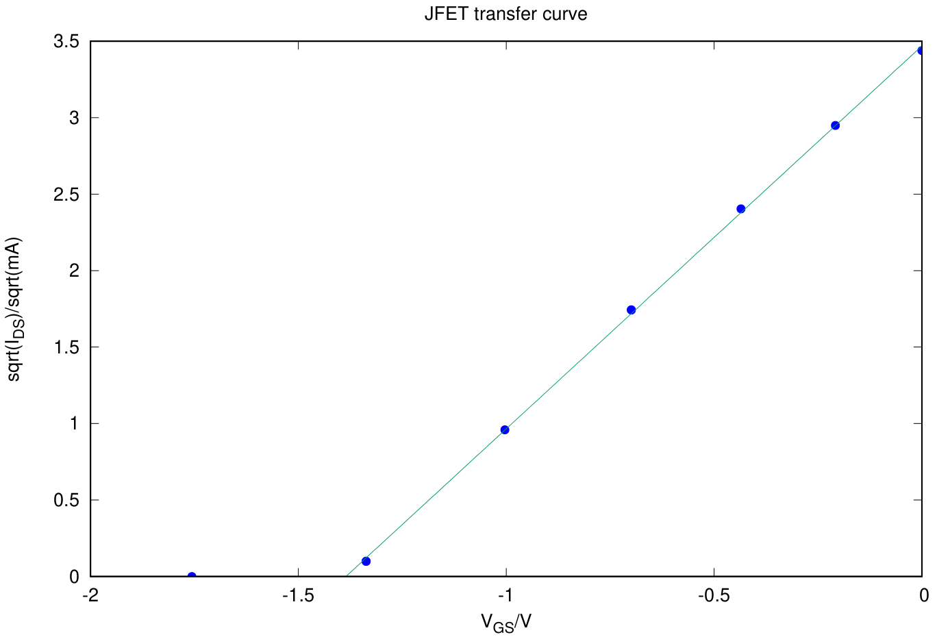
A linear fit to gave and . Thus, and .
B.8 (0.4 pt)
Source note: The source prints in the slope expression, without an opening parenthesis, and twice despite the stated intercept . These printed discrepancies are retained.
B.9
The transcondutance is the slope of the transfer curve at a given point. From the transfer plot, we draw the tangent at the point with abscissa and read the slope from the graph, obtaining .
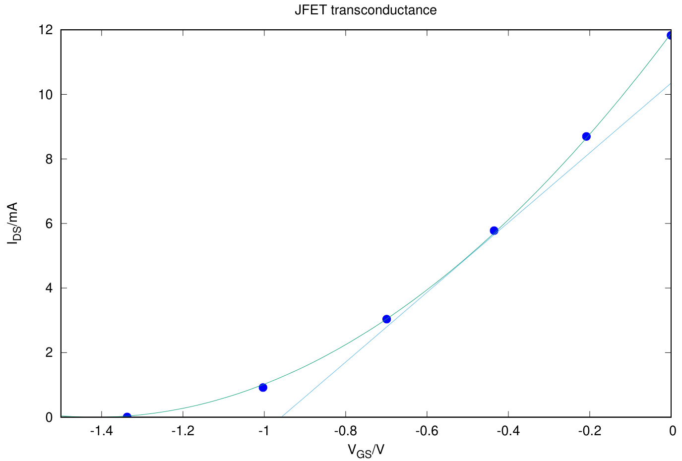
From
Substituting values,
a value that agrees with that obtained using the graphical method.
B.9 (0.4 pt)
Source note: The native key visibly prints “m” followed by the exponent for all these transconductance units; no ohm or siemens symbol is visible or present in the PDF text. The printed unit is retained without inserting a missing symbol. The starting equation uses , then the derivative uses .
Part C: The Paper Thin Film Transistor (2.0 points)
C.1 (0.8 pt)
| 0 | 0 | 110 | 112,0 |
| 10 | 6.6 | 120 | 116.2 |
| 20 | 25.8 | 180 | 137.7 |
| 30 | 50.1 | 240 | 155.4 |
| 40 | 66.2 | 300 | 171.2 |
| 50 | 76.7 | 360 | 184.4 |
| 60 | 83.8 | 420 | 197.9 |
| 70 | 91.6 | 480 | 209.2 |
| 80 | 97.2 | 540 | 219.1 |
| 90 | 102.6 | 600 | 220.0 |
| 100 | 107.4 | - | - |
C.2
The data is similar to that of the charge of a capacitor, superimposed with an almost linear component that corresponds to the charge of the second capacitor with a larger time constant.
A least squares fit to a is also depicted, showing that the data can be well fitted by this model. The shorter time constant is , the longer time constant, is roughly 20 times larger.
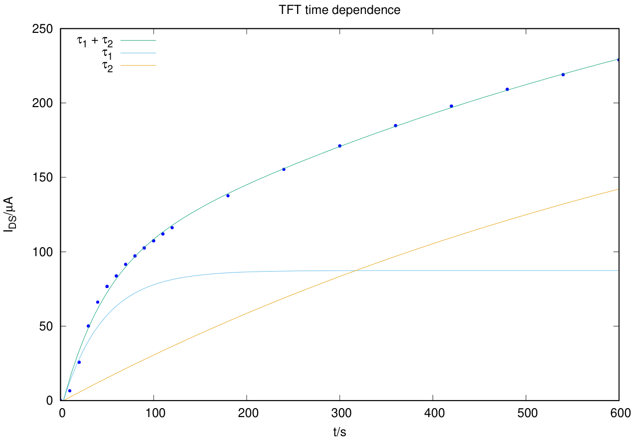
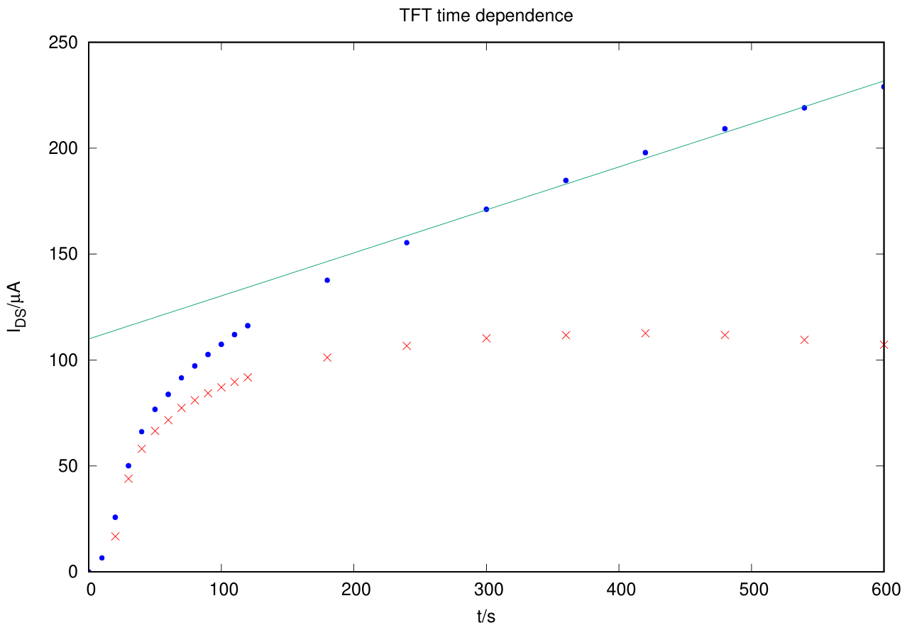
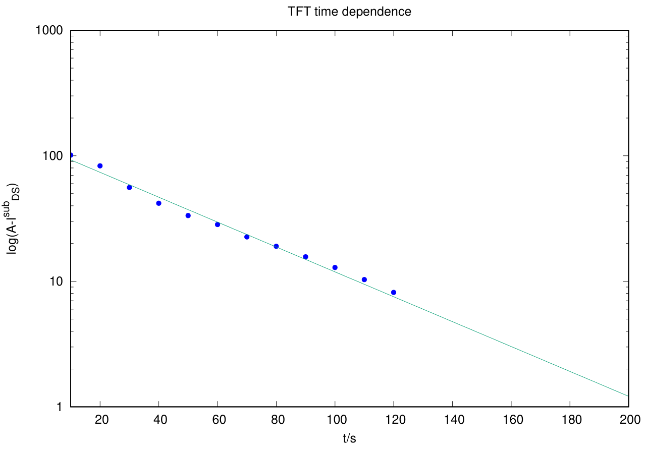
Let be the data subtracted from the long time constant component. A logarithmic plot of should be a straight line of slope . The constant , the saturation current of the short component, can be easily estimated from the above plot.
The slope of the line is , from which we get . The error bar is underestimated, as it does not take into account the error in the subtraction of the component.
C.2 (1.2 pt)
Part D. Inverter Circuit (1.0 points)
D.1 (0.5 pt)
| -2.983 | 2.456 | |
| -2.760 | 2.470 | |
| -2.567 | 2.461 | |
| -2.340 | 2.461 | |
| -2.058 | 2.460 | |
| -1.719 | 2.252 | |
| -1.330 | 0.889 | |
| -0.775 | 0.039 |
Source note: Every cell in this native key table is blank; no times are supplied here.
D.2 (0.5 pt)
Теми и трудност
Оценена трудност: 4/5.
Електричество · Съвременна физика · Постояннотокови вериги · Полупроводници · Преходни процеси в RC вериги
Предпоставки: Гимназиална подготовка, Разширена олимпиадна подготовка
Оригинал в Архива: exp1.pdf · официални решения: exp1_sol.pdf · допълнителни данни: exp1_anssheet.pdf