IPhO 2018, Експеримент — Задача 2. Viscoelasticity of a polymer thread
Viscoelasticity of a polymer thread (10 points) · 10 т.
Условие
Please note that the thread must not be stressed before the beginning of the experiment!
Switch on the scale right now (warming time is about 10 minutes). Do not change the settings of the scale.
Introduction
When a solid material is subject to an external force, it deforms. For small applied forces, this deformation is proportional to the force (Hooke's law) and is reversible, so that the material recovers its initial shape when the force is removed.
For a solid, the description is more conveniently expressed using the concepts of stress and strain. The stress is defined as the force per unit area, i.e. the force divided by the area on which it acts, whereas the strain, , is the relative change of length:
where and are the final and original length, respectively. In the simple elastic behaviour, the stress is simply proportional to the strain (Hooke's law) and the proportionality factor, , is named modulus of Young.
The elastic behaviour expressed in Hooke's law is an approximation valid only for small enough strains. For higher strains changes gradually become irreversible as the plastic regime is reached, in which case the molecular movements start to be unconstrained, resembling those of a viscous fluid. That is, if stretched or compressed beyond the elastic limit, the material becomes asymptotically fluid.
Viscoelastic materials
Certain materials combine aspects of an elastic solid with features resembling viscous fluids, and are therefore known as viscoelastic.
On dealing with a viscoelastic material it is reasonable to consider separately the purely elastic behaviour and the additional viscous behaviour, thus implying that the total stress needed to develop a given strain is the sum of a purely elastic term and a viscoelastic term :
Both stress terms are assumed to correspond to the same strain . However, the strain, , corresponding to the viscoelastic term is usually modelled as the sum of a purely elastic strain, , with a purely viscous strain, , (both subject to the same stress ):
In the purely viscous process, a linear relation between the stress and the time derivative of the strain is admitted (similarly to that found in viscous fluids),
where is the viscosity coefficient.
This phenomenological model is the so called standard linear solid model of linear viscoelasticity, and is depicted in Figure 1, where the springs represent pure elastic components and the pot represents the purely viscous component.
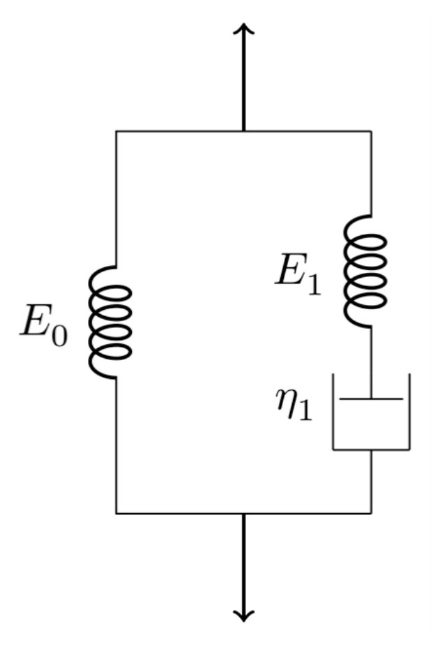
From the above equations the following relation is obtained:
Therefore, within the standard linear model of viscoelasticity, it is possible to show that
where . This differential equation shows that the relation between the strain and the stress is no longer linear, and that the strain and the stress are both in general functions of time. To get it is necessary to specify the function , and vice-versa.
There are two special cases of practical interest, in which either or , commonly known as the stress relaxation conditions and the creep conditions, respectively. Under the stress relaxation conditions, a sudden strain is applied to the material, which is kept constant over time, so that . In such a case, the function is then dependent only on the viscoelastic parameters of the medium and the solution of eq. (5) is
where it was admitted that at only the elastic components contribute to the stress and thus . This solution shows that the viscoelastic stress decays exponentially with time, with a time constant .
Multi-viscoelastic processes
The standard linear model can be readily extended to include many viscoelastic processes, as suggested by Figure 2.
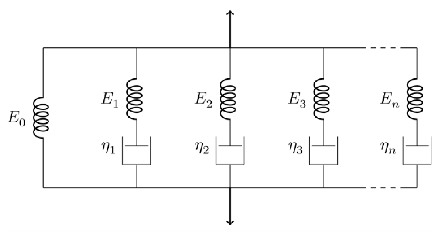
Thus, considering different viscoelastic components,
where , and as above, .
The following generalization of eq. (5) is thus applicable:
where , and .
In constant strain conditions, the various viscoelastic stresses should still decay exponentially with time, , leading to the solution:
where it was assumed that at only the elastic components contribute to the total stress and thus . The resulting viscoelastic response is evidently non-linear.
Equipment
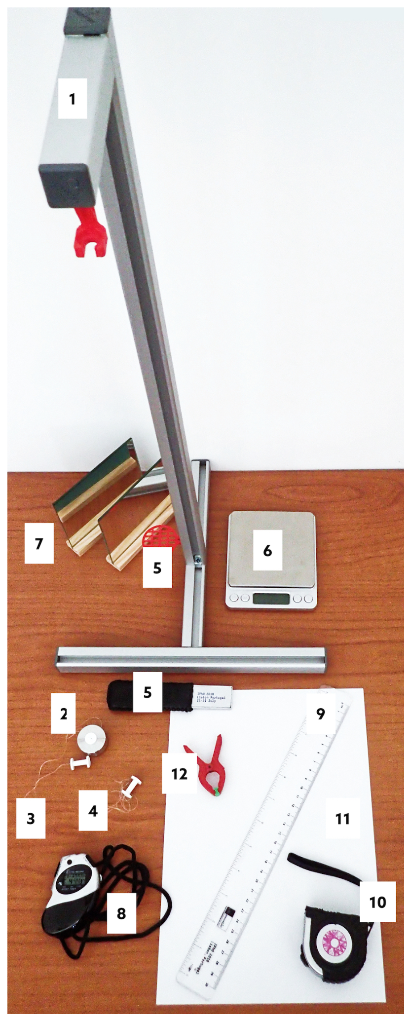
The following set of equipments is provided for this experimental problem (see Figure 3):
- 1 standing structure, with a supporting system to position a laser pointer and another upper supporting system to hold the thread stretched vertically with constant strain above the scale;
- 1 mass-set, consisting of a hollow cylindrical mass and a holding screw to attach the thread;
- 1 long thermoplastic polyurethane (TPU) thread attached to the mass-set and to another holding screw used to hang the thread from the upper support;
- 1 short TPU thread attached to a single holding screw;
- 1 laser pointer and the respective support;
- 1 digital scale;
- 2 plane mirrors;
- 1 stopwatch;
- 1 ruler;
- 1 metallic measuring tape;
- 1 sheet of A4 paper to act as a screen;
- 1 spring clamp to hold the laser in place and to switch it on.
Part A: Stress-relaxation measurements (1,9 т.)
Please note that the thread must not be stressed before the beginning of the experiment! In case the thread is inadvertently stressed, ask for a spare one, but be reminded that this will take some time, therefore reducing the time you have for your experiment.
You should read carefully the indications given on "Part D: Data Analysis" before starting the measurements on this part in order to plan the way you make the measurements.
A.1 Measure the length of the unstretched thread between the screw heads. To obtain the total thread length, , including the length inside the screws, add 5 mm for each screw. Write down in the answer sheet the measured value of and its uncertainty. [0,3 т.]
A.2 Measure the total weight of the mass-set, , in gram-force (gf) units. Remember that 1 gram-force is the force corresponding to the weight of a mass of 1 gram ( N). Write down in the answer sheet the measured value and an estimation of its uncertainty. [0,3 т.]
To observe experimentally the various relaxation components it is necessary to measure the stress for a long enough time. In this case, it is sufficient to sample the stress evolution during about 45 minutes.
You should now perform two simultaneous actions 1. and 2. Please read the instructions carefully before starting.
Important: if the experiment is interrupted for any reason it cannot be resumed. It has to be restarted with a new thread. In such case, ask for a spare one.
Take the following simultaneous actions:
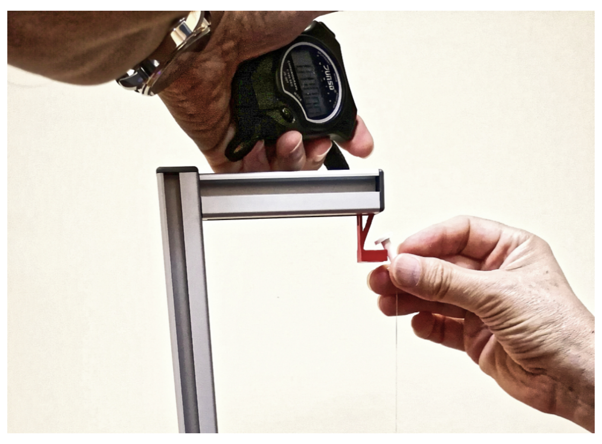
- Keeping the mass-set on the scale platform, stretch the thread so that the holding screw at the opposite side is placed on the thread supporting system, at the standing structure (Figure 4).
- Start the chronometer simultaneously with action 1.
A.3 Record the readings of the scale, , and the corresponding reading instant, , during around 45 min, in the table provided in the answer sheet. [1 т.]
A.4 Measure the length of the stretched thread, , and estimate the corresponding uncertainty. Write down in the answer sheet the measured value of and its uncertainty. [0,3 т.]
Part B: Measurement of the stretched thread diameter (1,5 т.)
Never look directly at the laser! When not in use, the laser pointer should be off.
If you have difficulties in getting a diffraction pattern, please ask for a new laser.
In this part you will use light diffraction to measure the diameter of the polymer thread. The nominal diameter of the unstretched thread is mm. As you may know, the diffraction pattern of a rectangular slit of width is similar to that of a cylindrical object with the same diameter as the slit width. In the far-field (Fraunhofer) regime, where the diffraction pattern is observed in a target screen placed at a distance much larger than the diameter of the object, the distance between the diffraction minima for small angles is the same for both the slit and the object and is given by
where is the diffraction angle.
You will use laser light with a wavelength = nm.
To perform this part, proceed as follows:
- Turn on the laser using the spring clamp (see Figure 5).
- Position the laser so that it hits the stretched thread directly.
- With the provided material, devise a method to project the diffraction pattern into a paper screen, and to measure the data needed to determine the diameter of the thread using eq. (10).
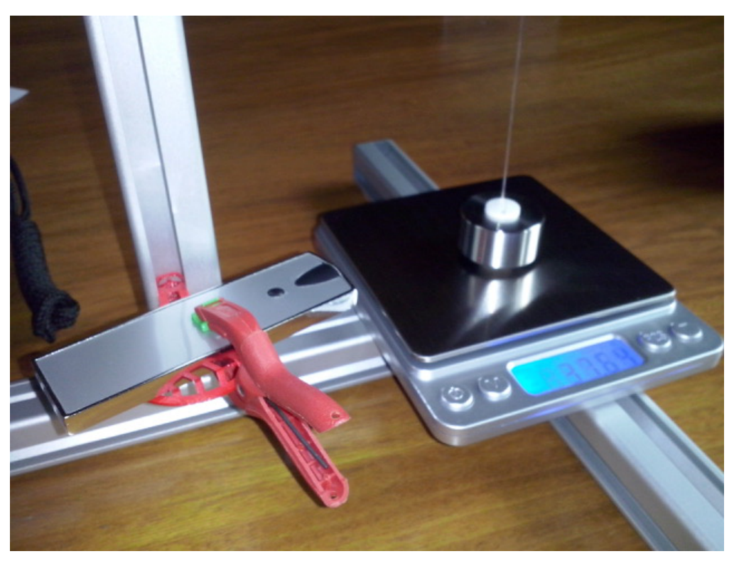
B.1 Make a sketch of your method in the answer sheet. [0,6 т.]
B.2 Measure the optical distance, , between the thread and the projected diffraction pattern. Write it down in the answer sheet with an estimation of its uncertainty. [0,3 т.]
B.3 Determine the average distance, , between diffraction minima and its uncertainty. Write it down in the answer sheet with an estimation of its uncertainty. [0,3 т.]
B.4 Applying eq. (10) to your diffraction data, determine the diameter, , of the stretched polymer thread and its uncertainty. Write it down in the answer sheet with an estimation of its uncertainty. [0,3 т.]
Part C: Changing to a new thread (0,3 т.)
Before proceeding with the data analysis (Part D) you have to prepare the setup for the measurement with the shorter thread (Part E).
Detach the mass-set from the long thread (unscrewing it) and transfer it to the free end of the shorter thread (inserting the thread through the hole and fixing it with the screw-thread, see Figure 6).
In case you are unable to insert the thread through the hole, please ask for help.
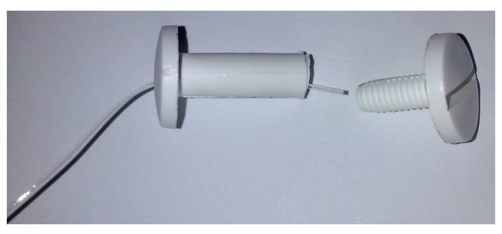
C.1 Measure the length, of the thread as in A.1. Write it down in the answer sheet with an estimation of its uncertainty. [0,3 т.]
Hang this new thread on the upper support so that the mass will exert a constant stress. The thread will eventually reach the stationary strain , while you work out the data analysis (it should be suspended for at least 30 minutes).
Part D: Data analysis (5,7 т.)
N.B.: The acceleration of gravity in Lisbon is .
D.1 Calculate the force on the thread, , in gf, for all data points and fill the corresponding column in the table used in A.3. [0,3 т.]
D.2 Plot in the graph paper provided in the answer sheet. [0,4 т.]
Since the scale platform does not move, the measurements can be considered at constant strain and eq. (9) can be used. The ratio can be written as , where is a constant. Therefore,
where the sum was ordered for convenience.
D.3 Determine the constant strain, , and the corresponding uncertainty. Write it down in the answer sheet with an estimation of its uncertainty. [0,3 т.]
D.4 Calculate the factor , with in SI units and in gf units. Write it down in the answer sheet (no uncertainty required). [0,3 т.]
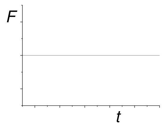
D.5 Look at the data in the graph used in D.2: it cannot be explained by a purely elastic process. Sketch qualitatively in the graph paper provided in the answer sheet what you would expect for in the purely elastic case. [0,4 т.]
The data analysis is easier if we consider instead of . This means that the relaxation parameters can then be extracted by hand in successive steps. In order to do this, the time derivative should be calculated at every point. This can be done either graphically or numerically. In the simpler case where the data points are taken at equal intervals, the numerical value of the derivative of a function at point , in a data set , is approximately given by
where is the (constant) interval between the points and is the number of points.
If the intervals between data points are not equal, the numerical value of the derivative is approximately given by:
where and and is the number of data points. This expression represents the average derivative at left and right, weighted by the inverse time interval.
To analyse the data and extract the relevant parameters it is necessary to follow a sequence of steps. Hence, given the ordered sum in equation (11), do the following:
D.6 Assume that your data set lasts for longer than and calculate the derivative, , for data points at times s. Register the values in the table used in A.3. In case you use a graphical method for calculating , use the graph paper provided in the answer sheet. [0,5 т.]
D.7 In the answer sheet, write an expression for the expected time dependence of in the case of a single viscoelastic process. [0,3 т.]
D.8 Extract, using a graphical method, the parameters and in SI units from the data points referred in D.6. Write and in the answer sheet (no uncertainties required). [1 т.]
D.9 Extract the parameter in SI units from the data points referred in D.6. Write it down in the answer sheet (no uncertainty required). [0,3 т.]
D.10 Fill column in the table used in A.3 by subtracting the elastic and the longest viscoelastic components from (the points used in D.6 do not need to be considered here). [0,3 т.]
D.11 Extract from (see D.10), using a graphical method, the parameters for the second viscoelastic component, and , in SI units. Write and in the answer sheet (no uncertainties required). [1 т.]
Additional viscoelastic components can be extracted in a similar way.
D.12 Identify the time window relevant for the third component. Write and in the answer sheet (no uncertainties required). [0,3 т.]
D.13 Estimate in SI units from the graph in D.11. Write it down in the answer sheet (no uncertainty required). [0,3 т.]
Part E: Measuring in constant stress conditions (0,6 т.)
Go back to the shorter thread suspended in Part C. Make sure that at least 30 minutes have passed since the thread was suspended. You can now safely assume that this thread has reached the stationary value of the strain .
E.1 Determine directly from the length of the stretched thread. Write it down in the answer sheet, together with the relative difference to the value obtained in Part D (no uncertainties required). [0,6 т.]
Отговори
Part B: Measurement of the stretched thread diameter, B.4 0.48 mm
Official sample result d = (0.480 ± 0.012) mm; the value depends on the student's own measurements.
Part D: Data analysis, D.4 324000 gf⁻¹ N m⁻²
Official sample result β = 3.24 × 10⁵ gf⁻¹ N m⁻²; the value depends on the student's own measurements.
Part D: Data analysis, D.9 N m⁻²
Official sample result E0 = 1.31 × 10⁷ N m⁻²; the value depends on the student's own measurements.
Part D: Data analysis, D.13 50 s
Official sample estimate τ3 ≈ 50 s.
Part E: Measuring in constant stress conditions, E.1 E = 1.337 × 10⁷ N m⁻², (E − E0)/E0 = 2.1%
Official sample result; depends on the student's own measurements.
Решение
Solutions to Experimental Problem 2
Viscoelasticity of a polymer thread
(J. M. Gil, J. Pinto da Cunha, R. C. Vilão, H. V. Alberto)
July 22, 2018
v1.1
Problem 2: Viscoelasticity of a polymer thread (10 points)
Part A. Stress-relaxation measurements (1,9 т.)
A.1 Measurement: cm ,
A.1 0.3pt
[0,3 т.]
A.2 A.2 0.3pt
[0,3 т.]
A.3 The table contains the readings on the scale (Question A.3) and the force on the thread, , at constant strain (Question D.1). The values of (Question D.6) were computed numerically using equal time intervals. The function is given by (Question D.10).
A.3 1.0pt
| /s | /gf | /gf | /gf s | /gf |
|---|---|---|---|---|
| 10 | 35.7 | 45.41 | 2.82 | |
| 17 | 36.2 | 44.91 | 2.33 | |
| 26 | 36.6 | 44.51 | 1.95 | |
| 32 | 36.8 | 44.31 | 1.76 | |
| 40 | 37.0 | 44.11 | 1.57 | |
| 46 | 37.1 | 44.01 | 1.48 | |
| 51 | 37.2 | 43.91 | 1.38 | |
| 58 | 37.3 | 43.81 | 1.29 | |
| 65 | 37.4 | 43.71 | 1.20 |
A.3 0.3pt
| /s | /gf | /gf | /gf s | /gf |
|---|---|---|---|---|
| 73 | 37.5 | 43.61 | 1.12 | |
| 84 | 37.6 | 43.51 | 1.03 | |
| 94 | 37.7 | 43.41 | 0.94 | |
| 105 | 37.8 | 43.31 | 0.86 | |
| 118 | 37.9 | 43.21 | 0.77 | |
| 136 | 38.0 | 43.11 | 0.70 | |
| 151 | 38.1 | 43.01 | 0.62 | |
| 173 | 38.2 | 42.91 | 0.55 | |
| 193 | 38.3 | 42.81 | 0.48 | |
| 217 | 38.4 | 42.71 | 0.41 | |
| 247 | 38.5 | 42.61 | 0.35 | |
| 279 | 38.6 | 42.51 | 0.29 | |
| 317 | 38.7 | 42.41 | 0.23 | |
| 358 | 38.8 | 42.31 | 0.18 | |
| 408 | 38.9 | 42.21 | 0.14 | |
| 471 | 39.0 | 42.11 | 0.11 | |
| 525 | 39.1 | 42.01 | 0.07 | |
| 591 | 39.2 | 41.91 | 0.03 | |
| 600 | 39.2 | 41.91 | 0.04 | |
| 672 | 39.3 | 41.81 | 0.01 | |
| 773 | 39.4 | 41.71 | 0.007 | |
| 866 | 39.5 | 41.61 | −0.01 | |
| 900 | 39.52 | 41.59 | −0.00 | |
| 993 | 39.6 | 41.51 | −0.01 | |
| 1124 | 39.7 | 41.41 | ||
| 1200 | 39.74 | 41.37 | ||
| 1272 | 39.8 | 41.31 | ||
| 1419 | 39.9 | 41.21 | ||
| 1500 | 39.94 | 41.17 | ||
| 1628 | 40.0 | 41.11 | ||
| 1800 | 40.06 | 41.05 | ||
| 1869 | 40.1 | 41.01 | ||
| 2037 | 40.2 | 40.91 | ||
| 2100 | 40.22 | 40.89 | ||
| 2400 | 40.29 | 40.82 |
[1 т.]
A.4 Measurement: cm ,
A.4 0.3pt
[0,3 т.]
Part B. Measurement of the stretched thread diameter (1,5 т.)
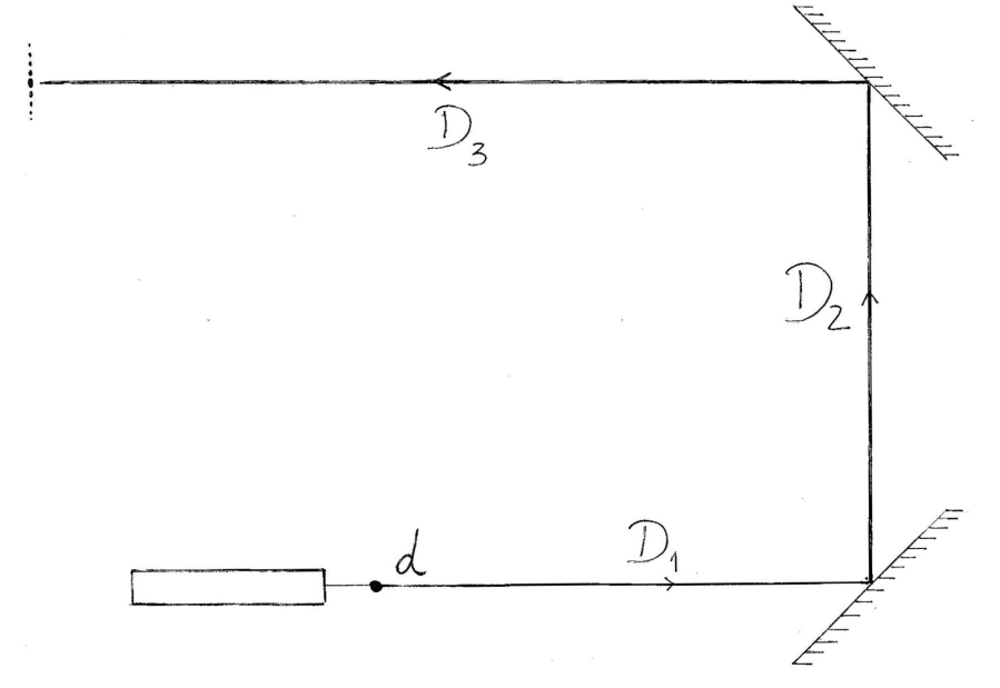
B.1 Two mirrors are used to maximize the distance D and consequently the distance between diffraction minima.
B.1 Sketch of the method 0.6pt [0,6 т.]
B.2 The total distance is the sum
The estimated uncertainties are
B.2 0.3pt
[0,3 т.]
B.3 The distance between minima, , is quite small. To reduce the error, the total distance , with , was measured:
The corresponding uncertainty is
B.3 0.3pt
[0,3 т.]
B.4 Using previous results, we get
For the uncertainties, we have
B.4 0.3pt
[0,3 т.]
Part C. Change to a new thread (0,3 т.)
C.1 Measurement: cm.
C.1 0.3pt
[0,3 т.]
Part D. Data Analysis (5,7 т.)
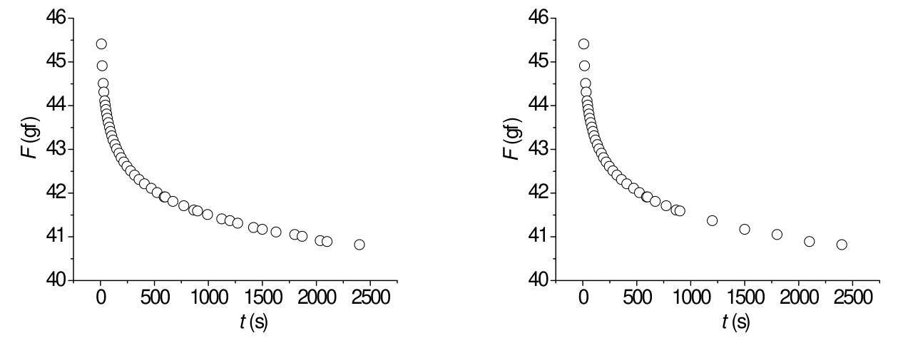
D.1 The force on the thread was calculated as , in gram-force units.
D.1 See column in the table in A.3. 0.3pt [0,3 т.]
D.2 D.2 0.4pt [0,4 т.]
D.3 The dimensionless quantity is given by
The uncertainty in , , is calculated propagating the uncertainties in the measured length, and :
Therefore, .
D.3 0.3pt
[0,3 т.]
D.4 One has
In this case, and . We also have with . Therefore, if is in gram-force units we have
where is in gf , and is in . Comparing with we get
Note that, if we write
and compare with equation
we conclude that , , , etc.
D.4 0.3pt
[0,3 т.]
D.5 For a purely elastic process, and
Thus, a graph of a constant function is expected.
D.5 0.4pt [0,4 т.]
D.6 The data for inserted in table introduced in A.3, was computed numerically for equal time intervals.
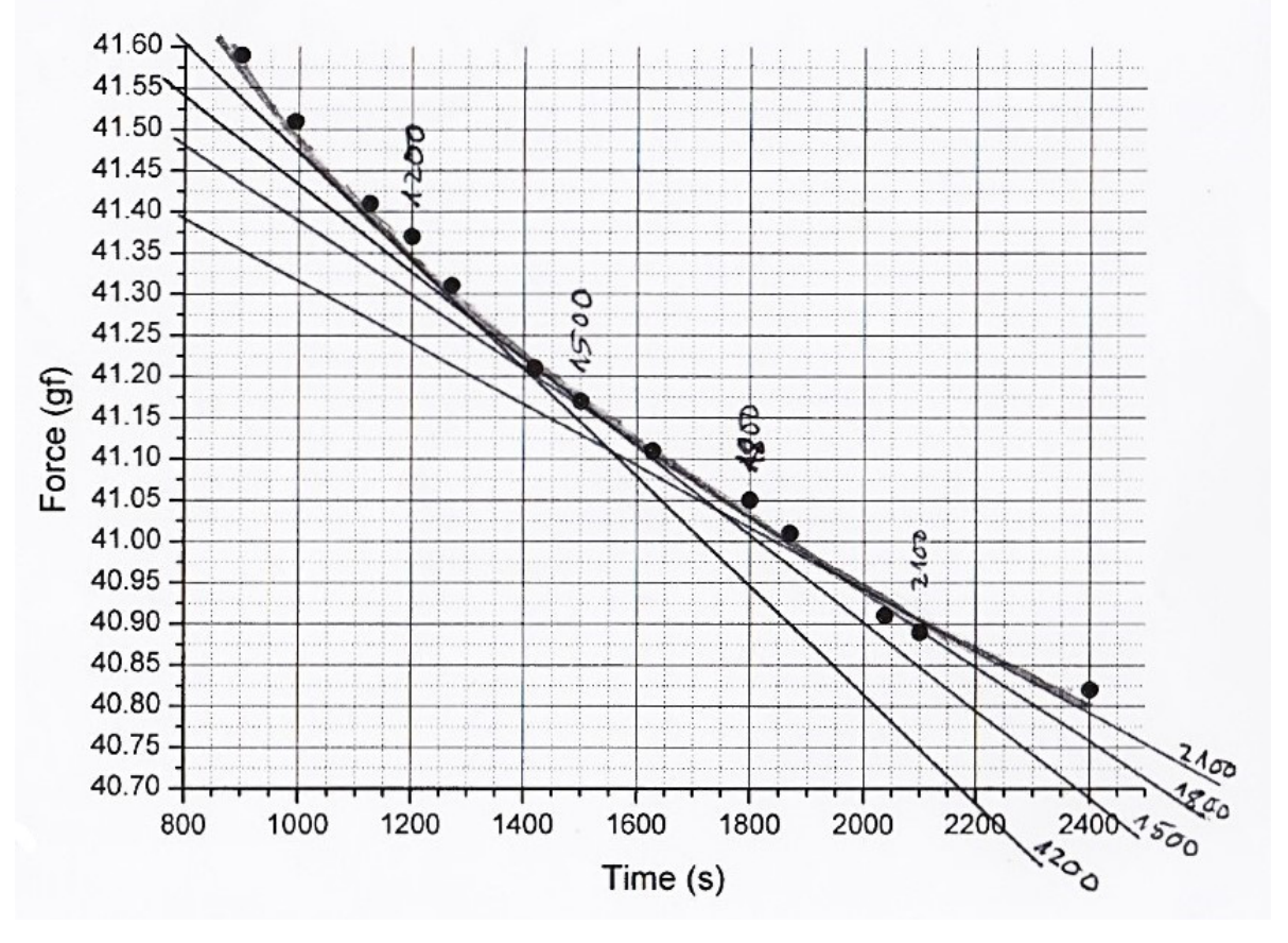
However, the graphical method is also exemplified. In the present graph, tangent lines to are drawn at four different time instants (1200,1500,1800 and 2100 s). The slopes of those lines are a measure of at those instants.
D.6 See in the table used in A.3, the column with . 0.5pt [0,5 т.]
D.7 For a single viscoelastic process,
Therefore,
D.7 0.3pt
[0,3 т.]
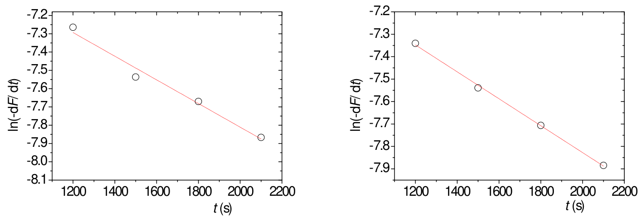
D.8 The linearisation of the expression of is accomplished using logarithms:
The plot of is shown in the graph below for a case where the derivative was obtained numerically (left) and using a graphic method (right).
For the left graph, the best straight line is where and , using in seconds and the force in gram-force units. If the derivative is computed numerically for unequal time intervals, the final parameters and are similar.
The best straight line for the right graph yields and using in seconds and the force in gram-force units.
Thus, using the data from the left graph, s and
For the right graph, the final parameters are s and .
D.8 1.0pt
[1 т.]
D.9 For the 4 points on the left graph in D.8, we can write
Thus, averaging for the 4 points of the left graph in D.8:
Finally,
D.9 0.3pt
[0,3 т.]
D.10 The function is given by
and was added in the Table introduced in A.3 using gf , gf and s.
D.10 See column in the Table in A.3. 0.3pt [0,3 т.]
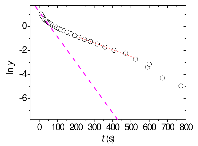
D.11 Since
then
At long times, when the contributions from the higher components are small enough, we expect a linear behaviour for :
In this case, the data points become meaningless above 500 s. In the region 200-500 s the graph is linear and that region can be used to extract the parameters of the second component. The equation of the straight line is . From the graph below,
.
D.11 1.0pt
The best straight line in the range 200-500 s yield the parameters and (Question D.11). The slope of the best straight line in the range s give an estimate of (Questions D.12 and D.13). [1 т.]
D.12 Below around 30 s there is clear deviation from a linear behaviour indicating the presence of a third component. In our case, the first data point was acquired at s.
D.12
[0,3 т.]
D.13 Drawing a line in the graph using the first data points (in the range defined in D.12), as shown in the graph in D.11, can be estimated as:
D.13 0.3pt
[0,3 т.]
Part E. Measuring in constant stress conditions (0,6 т.)
E.1 From Question C.1 we have
The final length should be measured. In our case,
Therefore, the strain is
Given that
Note that the radius of the stretched thread was not measured. We used the value measured in task B.4: m.
The relative difference is
E.1 0.6pt
[0,6 т.]
Оригинал в Архива: exp2.pdf · официални решения: exp2_sol.pdf