IPhO 2022, Експеримент — Задача 1. Planet
Experiment Q1 — Planet (12 points) · 12 т.
Условие
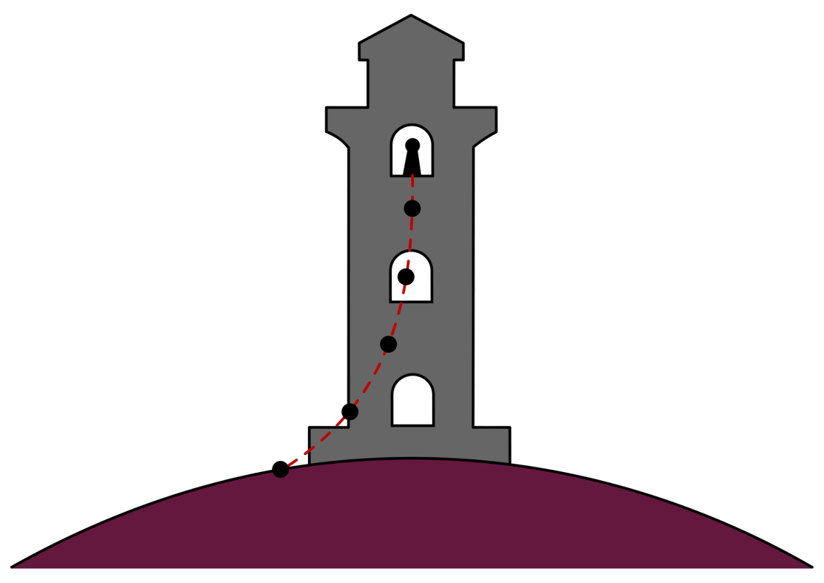
You find yourself on an alien planet with no knowledge of how you got there. The first thing you try to do is to learn more about the planet you're on. You remember how Galileo experimented with falling balls and inspired by this, build a perfectly vertical tower of height . Given the tower, you can now start dropping balls from any height on the tower (measured between the ground and the bottom of the ball immediately before it's released). Due to the limitations of the materials available to you, you can only drop balls of radius and densities .
Any time you drop a ball, you let it go from rest, and are able to measure the duration over which it falls, and the horizontal distance between where the ball lands and the point below where the ball was dropped.
Before you start your experiments, you make the following observations about the planet:
- Based on the movement of the Sun, you find that you're somewhere on the equator of the planet.
- The planet has an atmosphere; the air density is small enough for neglecting the buoyancy force due to it.
- The ground temperature is .
- There seems to be a wind blowing along the equator that's uniform throughout the height of the tower; neglect the effect of the tower on the wind velocity.
Description of the simulation software
The command line program simulates the measurements of the fall time and deflection from the base of the tower , after providing the height at which the ball is dropped, its radius , and density . All values of the input parameters are entered through the keyboard after the corresponding prompts and are validated by pressing the Enter key.
In order to get started, use the following authorization key when prompted:

Entering an incorrect value will put the program into test mode; you will need to restart the program.
A typical output of a single simulation cycle of the program looks like:
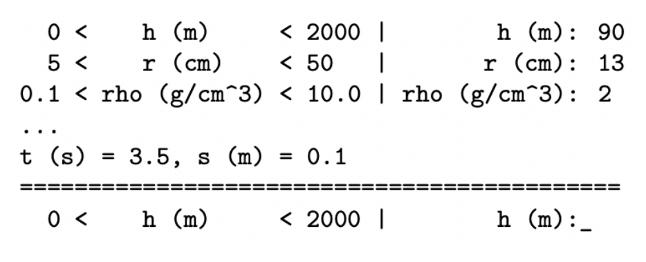
First, you enter the height in m (the number between 0 and 2000), then the radius of the ball in cm (the number between 5 and 50) and finally the density of the ball in g/cm (the number between 0.1 and 10). Each input is confirmed with the Enter key. The program will then output in s and in m.
The program then loops back to the height of the tower query.
Entering a value that is out of range for the experiment will result in an error message,
and then return you to the incorrectly answered prompt.

The height input will be rounded to 1 m, to 1 cm and to 0.01 g/cm. (There is no point in trying to input more precise numbers).
The results of the experiment will have random errors associated with them, as to simulate the limited precision one would have in real life. The sizes of the errors can be found by observing the fluctuations in the output.
Any time you need to quit the program, press Ctrl+C.
List of constants and useful relations
The gravitational constant .
Ideal gas constant ,
.
The air drag of a ball of cross-sectional area and speed in air of density is given by
An adiabatic atmosphere has a density profile given by
valid until the top of the atmosphere where K. Here, is the adiabatic coefficient, the molar mass of air (i.e. the gas in the atmosphere of the planet), the free-fall acceleration and the height from the ground.
Part A. Planetary properties (3.0 points)
A.1 Determine the free-fall acceleration on the planet by making a suitable set of measurements and sketching an appropriate graph in the space provided. Provide an analysis of the uncertainty in your result. [2 т.]
A.2 Walking away from the tower along the equator, you find that you can see the tower up to a distance of km away (measured as the distance between you and the top of the tower). What is the radius of the planet? You may assume that your height is much smaller than the height of the tower. [0,5 т.]
A.3 Estimate the mass of the planet. Provide an analysis of the uncertainty in your result.
What physical effect contributes the most to the accuracy of your estimate for ? Tick the appropriate effect the answer sheet. [0,5 т.]
Part B. Atmospheric properties (6.5 points)
B.1 Determine the wind speed on the surface of the planet by making a suitable set of measurements and sketching an appropriate graph in the space provided. Provide an analysis of uncertainty in your result. [2 т.]
B.2 Determine the air density on the surface of the planet either by collecting additional data or by reusing previous data, and sketching an appropriate graph in the space provided. Provide an analysis of the uncertainty in your result. [1 т.]
B.3 Assuming the atmosphere to be adiabatic with an adiabatic coefficient , determine the thickness of the atmosphere by making a suitable set of measurements and sketching an appropriate graph in the space provided. Provide an analysis of the uncertainty in your result. [3 т.]
B.4 Determine the molar mass of the air and the air pressure at the base of the tower. Provide an analysis of the uncertainty in your result. [0,5 т.]
Part C. Duration of a day (2.5 points)
C.1 Determine the duration of a day, , on the planet by making a suitable set of measurements and sketching an appropriate graph in the space provided. Provide an analysis of the uncertainty in your result. [2,5 т.]
Отговори
A.1 15.7 m/s²
Official value g = 15.7 m/s² with Δg = 0.5 m/s²; the marking scheme gives full marks for 15.0–16.4 m/s².
A.2 ≈ km
A.3 kg
Official: M = gR²/G = 4.2 × 10²⁵ kg with ΔM = 0.2 × 10²⁵ kg; the effect is the centrifugal force due to the planet's rotation, which reduces the measured acceleration and hence the estimate of M.
B.1 1.31 m/s
Official value u = 1.31 m/s with Δu = 0.04 m/s.
B.2 0.6 kg/m³
Official value ρa0 = 0.60 kg/m³ with Δρa0 = 0.07 kg/m³.
B.3 7500 m
Official value H0 = 7500 m with ΔH0 ≈ 2000 m.
B.4 μ = 72 g/mol ≈ 70 g/mol with Δμ = 20 g/mol; p0 = 20 000 Pa with Δp0 = 6000 Pa.
C.1 28000 s
Official value T = 28 000 s ≈ 8 h with ΔT = 0.2 h.
Решение
E1: Planet - SOLUTION
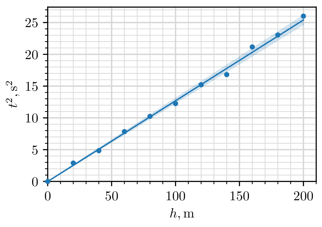
A.1: The free-fall acceleration can be found by dropping the ball from low heights such that the air friction and effects from the curvature of the planet are minimized. We also choose the radius and density of the ball to be as big as possible to minimize the effect of air friction, i.e. setting , . The drop height is then given by , and so we can find from the slope of vs . From the graph, we measure the slope and its error and so with an error of .
,
| 0 | 0.0 | 0.0 | 0.0 |
| 20 | 0.0 | 1.7 | 2.9 |
| 40 | 0.0 | 2.2 | 4.8 |
| 60 | 0.0 | 2.8 | 7.8 |
| 80 | 0.1 | 3.2 | 10.2 |
| 100 | 0.1 | 3.5 | 12.2 |
| 120 | 0.2 | 3.9 | 15.2 |
| 140 | 0.0 | 4.1 | 16.8 |
| 160 | 0.1 | 4.6 | 21.2 |
| 180 | 0.1 | 4.8 | 23.0 |
| 200 | 0.1 | 5.1 | 26.0 |
Marking scheme:
| Theory | 0.20 pts | |
|---|---|---|
| Data | varying only | 0.05 pts |
| maximising | 0.05 pts | |
| maximising | 0.05 pts | |
| table has units | 0.05 pts | |
| distributed roughly uniformly | 0.05 pts | |
| 0.05 pts | ||
| 0.05 pts | ||
| correct calculations of derived quantities | 0.05 pts | |
| 7 or more measurements | 0.30/0.30 | |
| 6 measurements | 0.25/0.30 | |
| 5 measurements | 0.20/0.30 | |
| 4 or fewer measurements | 0.10/0.30 | |
| Plotting | overall plot | 0.30 pts |
| points don’t cover 60% of the area | -0.10 pts | |
| missing axis labels | -0.05 pts | |
| missing axis units | -0.05 pts | |
| one plotting mistake | -0.05/-0.10 | |
| two or more plotting mistakes | -0.10/-0.10 | |
| Fit line | drawn on graph | 0.05 pts |
| line passes through origin | 0.05 pts | |
| slope computed with units | 0.10 pts | |
| uncertainty of slope computed | 0.10 pts | |
| Values | 0.20/0.20 | |
| 0.10/0.20 | ||
| units for value | 0.05 pts | |
| 0.20/0.20 | ||
| 0.10/0.20 | ||
| units for error | 0.05 pts | |
| sum | 2.0 pts |
Points are added additively (including negative points), except for blocks of grey background, where the option with maximal points should be chosen (in absolute value)
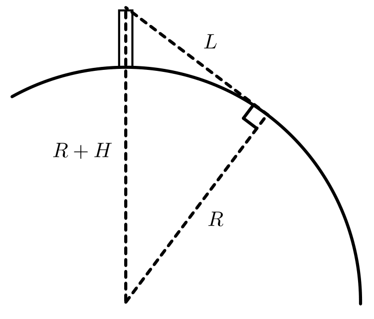
A.2: How far one can see from on top of the tower can be related to the radius of the planet via the right triangle shown in the figure below. Applying the Pythagoras theorem on the triangle, one gets and so
Marking scheme:
| Theory | correct geometry (either a figure or implicitly assumed) | 0.20 pts |
|---|---|---|
| correct formula | 0.20 pts | |
| Values | correct value | 0.10 pts |
| sum | 0.5 pts |
A.3: From Newton’s law of gravity, . Hence,
By adding the errors in quadrature, we find the error
Our estimation of free-fall acceleration has a contribution from the centrifugal force caused by the rotation of the planet. This serves to reduce the acceleration on the surface and hence decrease our estimation of the planet’s mass.
Marking scheme:
| Theory | correct formula | 0.10 pts |
|---|---|---|
| correct phenomena | 0.20 pts | |
| Values | 0.10/0.10 | |
| 0.05/0.10 | ||
| missing units for value | -0.05 pts | |
| 0.10/0.10 | ||
| 0.05/0.10 | ||
| missing units for error | -0.05 pts | |
| sum | 0.5 pts |
The student can’t get overall negative points for value nor error (for example when the value is completely out of range and the units are wrong).
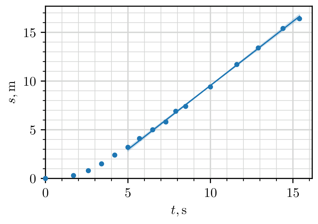
B.1: In general, if the variations in gravitational acceleration are small (as is the case here as ), as a response to air drag, objects tend to terminal velocity where they experience no net acceleration. In the reference frame of air, this corresponds to the object falling straight down with some terminal speed . In the lab frame, the object then has horizontal and vertical speeds of and respectively.
In order to find , we can choose to drop an object that reaches terminal velocity as fast as possible and then observe how the displacement relates to the fall time . When terminal velocity is reached, we expect , where captures the displacement related to reaching terminal velocity. To maximize the effects of air drag, we minimize radius and density, i.e. setting , and . Plotting vs , we measure the slope to be with an error of .
,
| 0 | 0.0 | 0.0 |
| 20 | 0.3 | 1.7 |
| 40 | 0.8 | 2.6 |
| 60 | 1.5 | 3.4 |
| 80 | 2.4 | 4.2 |
| 100 | 3.2 | 5.0 |
| 120 | 4.1 | 5.7 |
| 140 | 5.0 | 6.5 |
| 160 | 5.8 | 7.3 |
| 180 | 6.9 | 7.9 |
| 200 | 7.4 | 8.5 |
| 240 | 9.4 | 10.0 |
| 280 | 11.7 | 11.6 |
| 320 | 13.4 | 12.9 |
| 360 | 15.4 | 14.4 |
| 400 | 16.4 | 15.4 |
Marking scheme:
| Theory | idea of reaching terminal velocity as fast as possible | 0.15 pts |
|---|---|---|
| 0.10 pts | ||
| Data | varying only | 0.05 pts |
| minimising | 0.05 pts | |
| minimising | 0.05 pts | |
| table has units | 0.05 pts | |
| distributed roughly uniformly | 0.05 pts | |
| 0.05 pts | ||
| 0.05 pts | ||
| 7 or more measurements | 0.30/0.30 | |
| 6 measurements | 0.25/0.30 | |
| 5 measurements | 0.20/0.30 | |
| 4 or fewer measurements | 0.10/0.30 | |
| Plotting | overall plot | 0.30 pts |
| points don’t cover 60% of the area | -0.10 pts | |
| missing axis labels | -0.05 pts | |
| missing axis units | -0.05 pts | |
| one plotting mistake | -0.05/-0.10 | |
| two or more plotting mistakes | -0.10/-0.10 | |
| Fit line | drawn on graph | 0.10 pts |
| slope computed with units | 0.10 pts | |
| uncertainty of slope computed | 0.10 pts | |
| Values | 0.20/0.20 | |
| 0.10/0.20 | ||
| units for value | 0.05 pts | |
| 0.20/0.20 | ||
| 0.10/0.20 | ||
| units for error | 0.05 pts | |
| sum | 2.0 pts |
B.2: By keeping the measurements close to the surface, we can assume to a good approximation uniform air density. Then, using similar reasoning as before, we expect , where captures the part of reaching terminal velocity.
At terminal velocity, the drag force balances out gravitational acceleration:
Using and , we get
On the surface, . Using the measurements from the last subtask, we can plot vs and measure the slope to be with an error of . Hence, , . Now,
and the error is
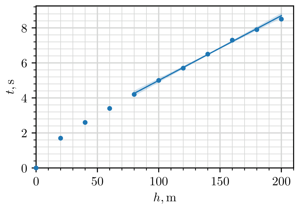
Marking scheme:
| Theory | 0.05 pts | |
|---|---|---|
| formula for terminal velocity | 0.10 pts | |
| final expression for | 0.05 pts | |
| Data | reusing the data from the last subpart | 0.05 pts |
| 0.05 pts | ||
| 6 or more measurements | 0.05 pts | |
| Plotting | overall plot | 0.25 pts |
| points don’t cover 60% of the area | -0.05 pts | |
| missing axis labels | -0.05 pts | |
| missing axis units | -0.05 pts | |
| one plotting mistake | -0.05/-0.10 | |
| two or more plotting mistakes | -0.10/-0.10 | |
| Fit line | drawn on graph | 0.05 pts |
| slope computed with units | 0.05 pts | |
| uncertainty of slope computed | 0.10 pts | |
| Values | 0.10/0.10 | |
| 0.05/0.10 | ||
| 0.10/0.10 | ||
| 0.05/0.10 | ||
| units for both value and error | 0.05 pts | |
| sum | 1.0 pts |
B.3: Due to the adiabatic profile of the atmosphere, the further up you go, the more the temperature and air density decreases, but the terminal velocity increases. We can estimate the terminal velocity of the ball at different heights by comparing the dropping time of a ball with the smallest possible terminal velocity (so minimal density and radius). This hence gives a direct probe for the air density and thus the height of the atmosphere.
If the ball reaches terminal velocity instantly, then the difference in falling time between dropping the ball at heights and comes simply from . This is because in both cases the ball falls for the same amount of time at (because the terminal velocity only depends on height). Then, if , we can estimate
In reality, the ball doesn’t reach the terminal velocity instantaneously. However, it turns out we can, to a good approximation, neglect this effect. As a rough order of magnitude estimation, on the ground level, the ball experiences a time difference of compared to the instantaneous case. This difference will increase as the ball is dropped from further up, but as long as the atmosphere isn’t too much sparser in the upper parts of the tower (we can verify this later), the difference will be insignificant compared to the total falling time of the ball. Hence, we approximate the terminal velocity via equation (1).
Because the calculated velocities are very sensitive on the measured quantities, we do repeated measurements throughout the whole height of the tower.
,
| 200 | 7.6 | 8.4 | 7.8 | 8.6 | 7.8 | 8.6 |
| 400 | 17.0 | 15.7 | 16.9 | 15.6 | 17.3 | 15.7 |
| 600 | 26.1 | 22.6 | 25.4 | 22.2 | 26.2 | 22.7 |
| 800 | 33.6 | 28.5 | 34.6 | 29.2 | 34.3 | 29.1 |
| 1000 | 41.1 | 34.3 | 43.0 | 35.7 | 43.3 | 35.8 |
| 1200 | 51.1 | 41.9 | 50.2 | 41.2 | 50.0 | 41.1 |
| 1400 | 57.9 | 47.2 | 58.8 | 47.8 | 58.7 | 47.8 |
| 1600 | 65.5 | 53.0 | 65.1 | 52.8 | 65.3 | 52.9 |
| 1800 | 70.9 | 57.1 | 72.2 | 58.2 | 71.4 | 57.5 |
| 2000 | 78.5 | 62.9 | 79.6 | 63.8 | 79.5 | 63.7 |
Using equation (1) we make a separate table with velocities, while also adding the ground level velocity found in one of the earlier part (we set it at because that was the centre of the range of measurements). We find air density using
From the density profile of an adiabatic atmosphere,
Hence, we find by plotting against and fitting a straight line.
,
| 100 | 27.0 | 0.599 | 0.814 |
| 300 | 28.0 | 0.556 | 0.791 |
| 500 | 29.3 | 0.510 | 0.764 |
| 700 | 31.1 | 0.452 | 0.728 |
| 900 | 31.6 | 0.438 | 0.719 |
| 1100 | 32.6 | 0.411 | 0.701 |
| 1300 | 32.3 | 0.420 | 0.707 |
| 1500 | 37.7 | 0.307 | 0.624 |
| 1700 | 42.6 | 0.241 | 0.566 |
| 1900 | 34.1 | 0.376 | 0.676 |
From the plot, we measure the slope and the intercept so . We calculate the error from two reasonably chosen lines that correspond to maximal and minimal estimates for
We can also confirm that our assumption about the density of the atmosphere not dropping significantly in the upper parts of the tower holds true.
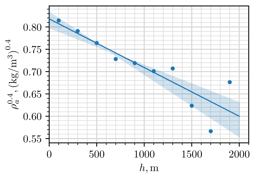
Marking scheme:
| Theory | approximating via finite difference | 0.30 pts |
|---|---|---|
| reasoning why the ball reaches terminal velocity effectively instantaneously | 0.15 pts | |
| linearising vs | 0.25 pts | |
| expressing in terms of the slope/intercept | 0.10 pts | |
| Data | varying only | 0.05 pts |
| minimising | 0.05 pts | |
| minimising | 0.05 pts | |
| table has units | 0.05 pts | |
| distributed roughly uniformly | 0.05 pts | |
| 0.10 pts | ||
| calculating derived quantities | 0.20 pts | |
| 15 or more measurements (can be repeat) | 0.45/0.45 | |
| 10 - 14 measurements | 0.30/0.45 | |
| 1 - 9 measurements | 0.15/0.45 | |
| Plotting | overall plot | 0.30 pts |
| points don’t cover 60% of the area | -0.10 pts | |
| missing axis labels | -0.05 pts | |
| missing axis units | -0.05 pts | |
| one plotting mistake | -0.05/-0.10 | |
| two or more plotting mistakes | -0.10/-0.10 | |
| Fit line | drawn on graph | 0.10 pts |
| slope computed with units | 0.15 pts | |
| uncertainty of slope computed | 0.15 pts | |
| Values | 0.20/0.20 | |
| 0.10/0.20 | ||
| units for value | 0.05 pts | |
| 0.20/0.20 | ||
| 0.10/0.20 | ||
| units for error | 0.05 pts | |
| sum | 3.0 pts |
B.4: From the expression for adiabatic atmosphere we have
so
and
From ideal gas law,
and
Marking scheme:
| Theory | correct expression for | 0.15 pts |
|---|---|---|
| correct expression for | 0.15 pts | |
| Values | 0.05 pts | |
| 0.05 pts | ||
| 0.05 pts | ||
| 0.05 pts | ||
| sum | 0.5 pts |
C.1: Our goal is to find the rotation speed of the planet. The rotation of the planet affects the ball’s trajectory via centrifugal and Coriolis force. The centrifugal force, however, due to is impossible to disentangle from gravitational acceleration. Coriolis force affects the ball via acceleration . This is perpendicular to both the velocity of the ball and rotation axis of the planet. Hence, it’s directed along the equator, and increases linearly with the falling speed. Thus, the horizontal acceleration is given by .
The procedure is then to minimize the effect of air drag (maximal radius and density) and hope that the Coriolis effect contributes enough to the horizontal displacement. If we neglect air drag, then so and . The final displacement will then be , where the falling time satisfies . Putting them together, we get
By varying the radius/density, we do indeed confirm that the effect of Coriolis force is significant, on the order of couple of meters. By doing a suitable number of measurements in the range to and plotting vs , we measure the slope
and the error
such that
and
,
| 0 | 0.0 | 0 |
| 200 | 0.2 | 2800 |
| 400 | 0.5 | 8000 |
| 600 | 0.8 | 14700 |
| 800 | 1.2 | 22600 |
| 1000 | 1.8 | 31600 |
| 1200 | 2.3 | 41600 |
| 1400 | 2.8 | 52400 |
| 1600 | 3.4 | 64000 |
| 1800 | 4.0 | 76400 |
| 2000 | 4.8 | 89400 |
Alternative solution.
An alternative approach is to consider the system in the non-rotating frame (where we don’t have to deal with fictitious forces). In there, the ball starts off with speed . Due to the conservation of angular momentum, as the ball drops towards the ground, the ball’s angular speed will start increasing and the ground will start lagging behind (the ground rotates with ). At height , when the ball moves with angular speed , the conservation of angular momentum reads and so the angular lag between the ball and the ground is
The positional velocity shift along the ground is then . We recover the same expression as for Coriolis force, and from there we proceed the same way as before.
Marking scheme:
| Theory | Deriving | 0.80 pts |
|---|---|---|
| linearising vs | 0.10 pts | |
| Data | varying only | 0.05 pts |
| minimising and | 0.05 pts | |
| table has units | 0.05 pts | |
| distributed roughly uniformly | 0.05 pts | |
| 0.05 pts | ||
| calculating derived quantities | 0.05 pts | |
| 7 or more measurements | 0.30/0.30 | |
| 6 measurements | 0.25/0.30 | |
| 5 measurements | 0.20/0.30 | |
| 4 or fewer measurements | 0.10/0.30 | |
| Plotting | overall plot | 0.30 pts |
| points don’t cover 60% of the area | -0.10 pts | |
| missing axis labels | -0.05 pts | |
| missing axis units | -0.05 pts | |
| one plotting mistake | -0.05/-0.10 | |
| two or more plotting mistakes | -0.10/-0.10 | |
| Fit line | drawn on graph | 0.10 pts |
| slope computed with units | 0.10 pts | |
| uncertainty of slope computed | 0.10 pts | |
| Values | 0.20/0.20 | |
| 0.10/0.20 | ||
| missing units for value | -0.05 pts | |
| 0.20/0.20 | ||
| 0.10/0.20 | ||
| missing units for error | -0.05 pts | |
| sum | 2.5 pts |
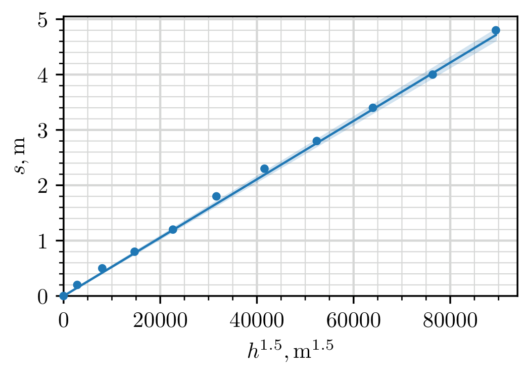
Оригинал в Архива: exam-experiment-Q1-english (1).pdf · официални решения: experiment_solutions (1).pdf