IPhO 2022, Експеримент — Задача 2. Cylindrical Diode
Experiment Q2 — Cylindrical Diode (8.0 pts) · 8 т.
Условие
Experimental setup and tasks
A cylindrical vacuum diode consists of two coaxial cylinders. There is an emitter of radius and length , which gives off electrons; these electrons travel through the vacuum to the collector, that has a radius and an effective infinite length. The collector is at a positive potential , while the emitter is grounded, so electrons are drawn from the emitter to the collector.
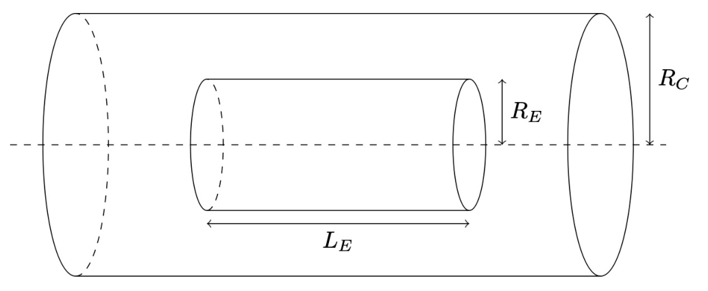
The emitter is heated so that there are always excess electrons available to be accelerated through the potential difference toward the collector. The electrons fill the vacuum with a plasma. Because of the properties of a plasma there is a maximum current that can flow through the diode that depends on the potential of the collector and the geometry of the system.
Throughout this experiment you should restrict your measurements to .
When is sufficiently large compared to it is hypothesized that the maximum current through the diode is
where is not a constant, but is instead a function of the dimensionless ratio .
When is comparable to it is necessary to issue a correction to the above expression, and the maximum current through the diodes is given by
where is a dimensionless function of some or all of , , , and . Equation (1) is the special case of Equation (2) when
In doing this experiment you have simulated access to any cylinder of radii 0.1 cm to a maximum of 20.0 cm, in steps of 0.1 cm; the cylinder lengths can be between 1.0 cm and 99.0 cm, also in steps of 0.1 cm. There is a simulated power supply that can provide a positive voltage to the collector between 0 and 2000 volts, and an ammeter that can measure the current through the diode.
You are encouraged to read all the tasks through quickly before beginning in order to plan your data collection more efficiently.
Description of the simulation software
The simulation program, named Exp2, allows users to perform an unlimited number of measurements of the maximum current for different sets of input parameters: the collector radius , the emitter radius and length and , and the potential difference between the emitter and the collector . All values of the input parameters are entered through the keyboard after corresponding prompts and validated by pressing the Enter key.
In order to get started, use the following authorization key when prompted:
Enter Valid Authorization Key: 12345678.888
Entering an incorrect value will put the program into test mode; you will need to restart the program.
A typical interface of a single simulation cycle of the program looks like:
0.1 < R_C (cm) < 20.0 | R_C (cm): 18.5
0.1 < R_E (cm) < 20.0 | R_E (cm): 13.2
0.1 < L_E (cm) < 99.0 | L_E (cm): 35.3
1.0 < V_C (V) < 2000.0 | V_C (V): 207

I (A) = 1.04
=======================================
0.1 < R_C (cm) < 20.0 | R_C (cm):
First you enter the collector radius, then the emitter radius, then the emitter length, each in centimeters, and finally the potential difference, in volts. Each input is confirmed with the Enter key.
The program then loops back to the collector radius query.
Entering a value that is out of range for the experiment will result in an error message,
Value Out Of Bounds
and then return you to the incorrectly answered prompt.
All lengths are only recorded to the nearest millimeter while all voltages are only recorded to the nearest volt; entering in a more precise number does not improve the measurement. However, there is an uncertainty of as much as 0.5 mm in any length, and 0.5 V in any voltage. As such, repeated measurements could give different results for the current.
The ammeter is auto-ranging, so that it shows only three significant figures, and switches between the amp or milliamp scale as appropriate. The uncertainty is of the last displayed digit. Pay attention to whether it is reporting in mA or A.
Exceeding the 40 amp current rating on the ammeter will burn it out. The program will notify you of this, and then automatically fix the ammeter for the next measurement.
Any time you need to quit the program in order to restart, press Ctrl+C.
Part A: Finding Exponents (4.5 pts)
Find the exponents in Eq (1), providing an analysis on error bounds on each result:
A.1 Collect a set of data that can be used to find the exponent on the variable . Sketch an appropriate graph in the space provided; for your convenience both linear and log-log graph paper is provided, but you only need to draw one graph. State your value of and provide an analysis of the uncertainty in your result. [1,5 т.]
A.2 Collect a set of data that can be used to find the exponent on the variable . Sketch an appropriate graph in the space provided; a single graph is sufficient. State your value of and provide an analysis of the uncertainty in your result. [1,5 т.]
A.3 Collect a set of data that can be used to find the exponent on the variable . Sketch an appropriate graph in the space provided; a single graph is sufficient. State your value of and provide an analysis of the uncertainty in your result. [1,5 т.]
Part B: Finding the Coefficient G (1.0 pts)
Find the value of the function when :
B.1 Either by collecting additional data or by reusing previous data, determine the value for when and provide an analysis of uncertainty in your result. [1 т.]
Part C: Finding dimensionless function F (2.5 pts)
Experimentally determine which of , , , and affect when is comparable to the size in Equation (2).
C.1 In the list of the variables on the answer sheet, state the direction of the effect; for example, does increase, decrease, or stay the same if is increased? [0,5 т.]
C.2 It is observed that when the function can be approximated as linear in a single variable , where is a function of only two from , , , and . The answer sheet has several possible functional forms for ; select the one that captures the most significant behavior. [0,5 т.]
C.3 Assume a linear function of the form for values of , and experimentally determine the parameter . Restrict to the range . Sketch an appropriate graph for in terms of your single appropriate quantity to approximate as a linear function. Error analysis is not necessary [1,5 т.]
Отговори
A.1 1.49
Official solution: best fit log I = 1.490 log V − 0.8095, γ = 1.490 ± 0.005 (statistical) or γ = 1.485 ± 0.025 (extreme lines).
A.2 0.98
Official solution: best fit slope 0.9767; β = 0.98 ± 0.02 (statistical) or β = 0.97 ± 0.02 (graphical).
A.3 -0.98
Official solution: best fit slope −0.9816, stated as α = −0.9824; the uncertainty lines print the symbol β ("β = −0.98 ± 0.01", "β = 0.97 ± 0.02") where α is meant.
B.1 0.0165 mA/V^(3/2)
Official solution: C = (0.0165 ± 0.0003) mA/V^(3/2) = 16.5 µA/V^(3/2) (the solution calls the coefficient C).
C.1 If RC increases, F increases; if LE increases, F decreases; V and RE have no significant effect on F.
C.2
Any multiple of RC/LE is also acceptable.
C.3 0.1762
Official fit F(x) = 0.8579 + 0.1762x; the marking scheme accepts 0.17 < B < 0.18.
Решение
Take the logarithm of Equation 1,
A.1: Collect data by varying . To minimize error, select maximum values for all fixed variables, this means cm, cm, and cm. Distribute the voltages logarithmically between 10 and 2000
| (V) | (mA) | ||
|---|---|---|---|
| 10 | 5 | 1.0 | 0.70 |
| 20 | 13 | 1.3 | 1.11 |
| 50 | 52 | 1.7 | 1.72 |
| 100 | 147 | 2.0 | 2.17 |
| 200 | 415 | 2.3 | 2.62 |
| 500 | 1620 | 2.7 | 3.21 |
| 1000 | 4630 | 3.0 | 3.67 |
| 2000 | 12900 | 3.3 | 4.11 |
Plot this on a graph; the best fit line is
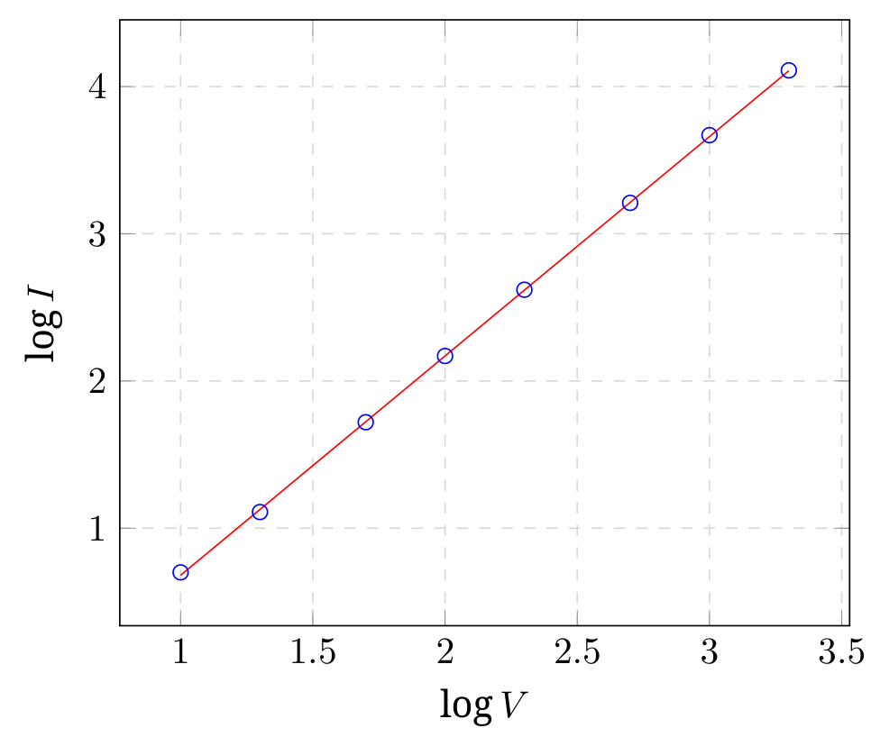
so .
A statistical analysis of the uncertainty in the slope yields .
Assessing the slope by visually fitting lines through the error bars on the points requires considering that error bars on a log axis are given by
Since the largest relative error is in the smallest valued quantity, the focus is on for and for . The error bars associated with the log-log plot at that point are then
The other error bars are smaller; focusing on that point alone we can fit two extreme lines and get
Either approach is acceptable.
Marking scheme:
| Data | vary only | 0.05 pts |
|---|---|---|
| cm | 0.05 pts | |
| cm | 0.05 pts | |
| cm | 0.05 pts | |
| table has units | 0.05 pts | |
| distributed as log | 0.05 pts | |
| V | 0.05 pts | |
| V | 0.05 pts | |
| V | 0.05 pts | |
| Correct calculations | 0.05 pts | |
| 7 or more points | 0.30/0.30 | |
| 6 points | 0.25/0.30 | |
| 5 points | 0.20/0.30 | |
| 4 or fewer points | 0.10/0.30 | |
| Plotting | covers % of area | 0.10 pts |
| Axis labels | 0.05 pts | |
| Axis units correct | 0.05 pts | |
| one plotting mistake | -0.05/-0.10 | |
| two or more plotting mistakes | -0.10/-0.10 | |
| Fit | line drawn on graph | 0.10 pts |
| slope correctly computed with units | 0.10 pts | |
| 0.10 pts | ||
| uncertainty of slope computed | 0.10 pts | |
| 0.10 pts | ||
| sum | 1.5 pts |
Measured data should be entered into spreadsheet that will calculate results; if deviation is too large, data point should not count.
Evidence of reverse engineering should result in zero points for the entire section
A.2: Collect data by varying . To minimize error, select maximum values for all fixed variables, this means V, cm, and cm.
| (cm) | (mA) | ||
|---|---|---|---|
| 99 | 13000 | 1.996 | 4.144 |
| 90 | 11800 | 1.954 | 4.072 |
| 80 | 10700 | 1.903 | 4.029 |
| 70 | 9170 | 1.845 | 3.962 |
| 60 | 7960 | 1.778 | 3.901 |
| 55 | 7310 | 1.740 | 3.864 |
| 50 | 6700 | 1.699 | 3.826 |
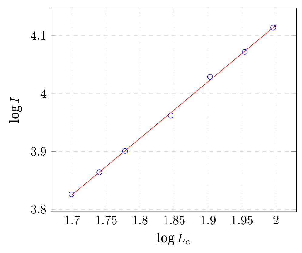
Plot this on a graph; the best fit line is
so .
A statistical analysis of the uncertainty in the slope yields .
Graphical fitting of the steepest and shallowest lines yields .
Marking scheme:
| Data | vary only | 0.05 pts |
|---|---|---|
| cm | 0.05 pts | |
| cm | 0.05 pts | |
| V | 0.05 pts | |
| table has units | 0.05 pts | |
| distributed evenly | 0.05 pts | |
| cm | 0.05 pts | |
| 0.05 pts | ||
| cm | 0.05 pts | |
| Correct calculations of derived quantities | 0.05 pts | |
| 7 or more points | 0.30/0.30 | |
| 6 points | 0.25/0.30 | |
| 5 points | 0.20/0.30 | |
| 4 or fewer points | 0.10/0.30 | |
| Plotting | covers % of area | 0.10 pts |
| Axis labels | 0.05 pts | |
| Axis units correct | 0.05 pts | |
| one plotting mistake | -0.05/-0.10 | |
| two or more plotting mistakes | -0.10/-0.10 | |
| Fit | line drawn on graph | 0.10 pts |
| slope correctly computed with units | 0.10 pts | |
| 0.10 pts | ||
| uncertainty of slope computed | 0.10 pts | |
| 0.10 pts | ||
| sum | 1.5 pts |
A.3: Collect data by varying . To minimize error, select maximum values for all fixed variables, this means V, cm, and cm.
| (cm) | (mA) | ||
|---|---|---|---|
| 20 | 6640 | 1.301 | 3.822 |
| 19 | 6970 | 1.279 | 3.843 |
| 18 | 7380 | 1.255 | 3.868 |
| 16 | 8240 | 1.204 | 3.916 |
| 14 | 9390 | 1.146 | 3.973 |
| 12 | 11000 | 1.079 | 4.041 |
| 10 | 13100 | 1.000 | 4.117 |
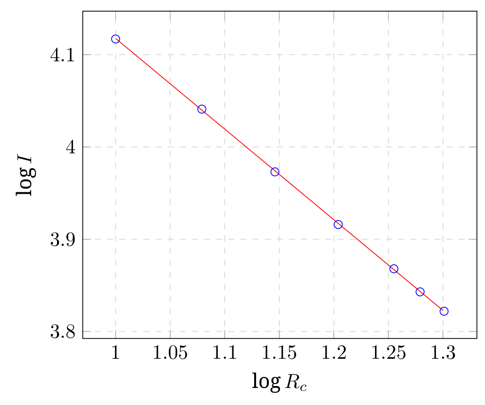
Plot this on a graph; the best fit line is
so .
A statistical analysis of the uncertainty in the slope yields .
Graphical fitting of the steepest and shallowest lines yields .
Marking scheme:
| Data | vary only | 0.05 pts |
|---|---|---|
| cm | 0.05 pts | |
| cm | 0.05 pts | |
| V | 0.05 pts | |
| table has units | 0.05 pts | |
| distributed evenly | 0.05 pts | |
| cm | 0.05 pts | |
| 0.05 pts | ||
| cm | 0.05 pts | |
| Correct calculations of derived quantities | 0.05 pts | |
| 7 or more points | 0.30/0.30 | |
| 6 points | 0.25/0.30 | |
| 5 points | 0.20/0.30 | |
| 4 or fewer points | 0.10/0.30 | |
| Plotting | covers % of area | 0.10 pts |
| Axis labels | 0.05 pts | |
| Axis units correct | 0.05 pts | |
| one plotting mistake | -0.05/-0.10 | |
| two or more plotting mistakes | -0.10/-0.10 | |
| Fit | line drawn on graph | 0.10 pts |
| slope correctly computed with units | 0.10 pts | |
| 0.10 pts | ||
| uncertainty of slope computed | 0.10 pts | |
| 0.10 pts | ||
| sum | 1.5 pts |
B.1: Use all three sets of data, and the exponents from all three, and then average the results
which gives
The theoretical value is approximately:
Note that there is a nasty correction (the texts usually call it , which is not the same as our exponent), that we use in the code, but aren’t expecting students to find, because of this correction, we don’t expect the theoretical value to hold. Students who try to solve the theoretical problem will be vexed by this.
For space reasons, we write numerical below without explicit units, but using the units of , that is
Students must have clear units!
Marking scheme:
| Theory | clear statement | 0.20 pts |
|---|---|---|
| Fit | Used | 0.10 pts |
| computed | 0.10 pts | |
| More than 9 data points | 0.20/0.20 pts | |
| 8 or 9 data points | 0.15/0.20 pts | |
| 7 or 8 data points | 0.10/0.20 pts | |
| 5 or 6 data points | 0.05/0.20 pts | |
| has correct units | 0.10 pts | |
| 0.10/0.10 pts | ||
| 0.05/0.10 pts | ||
| uncertainty computed | 0.10 pts | |
| 0.10 pts | ||
| 0.05/0.10 pts | ||
| sum | 1.0 pts |
Clear statement of theory means that somewhere there is a justification for the data they are collecting and using. This can be in the form of the log formula; words are not necessary. Reusing data is okay.
C.1: Start by assuming that matters, and look at values near . Repeat for other variables. Remember that depends on the ratio between , so change these together!
Using nearest half integers, we have for the first equation
so that
| cm | cm | cm | V | mA | mA | |
| 10 | 1 | 10 | 1000 | 535 | 500 | 1.071 |
| 12 | 1.2 | 10 | 1000 | 470 | 416 | 1.129 |
| 8 | 0.8 | 10 | 1000 | 647 | 624 | 1.036 |
| 10 | 1 | 12 | 1000 | 630 | 599 | 1.051 |
| 10 | 1 | 8 | 1000 | 451 | 400 | 1.129 |
| 12 | 1.2 | 12 | 1000 | 537 | 500 | 1.075 |
| 8 | 0.8 | 8 | 1000 | 537 | 500 | 1.075 |
| 10 | 1 | 10 | 1100 | 617 | 576 | 1.071 |
| 10 | 1 | 10 | 900 | 457 | 426 | 1.072 |
From this we conclude that if , ; if , ; if , doesn’t change.
Also, we notice that the ratio seems to be the important quantity.
Marking scheme:
| Data | clearly collected | 0.10 pts |
|---|---|---|
| Data | 0.10 pts | |
| 0.10 pts | ||
| : no significant change | 0.10 pts | |
| : no significant change | 0.10 pts | |
| sum | 0.5 pts |
C.2: We propose
with .
Marking scheme:
| Theory | clear statement | 0.20 pts |
|---|---|---|
| Def | 0.30/0.30 pts | |
| 0.15/0.30 pts | ||
| sum | 0.5 pts |
Any multiple of is also acceptable.
C.3: It is important to collect data that varies and independently, so as to not bias our hypothesis. We will also keep the ratio with , in order to avoid other effects with the constant in part B.
| (cm) | (cm) | (mA) | |||
|---|---|---|---|---|---|
| 20 | 10 | 898 | 740 | 2.000 | 1.213 |
| 20 | 15 | 1210 | 1110 | 1.333 | 1.090 |
| 20 | 20 | 1520 | 1480 | 1.000 | 1.027 |
| 20 | 30 | 2160 | 2221 | 0.667 | 0.973 |
| 20 | 40 | 2810 | 2961 | 0.500 | 0.949 |
| 6 | 10 | 2420 | 2467 | 0.600 | 0.981 |
| 8 | 10 | 1840 | 1850 | 0.800 | 0.994 |
| 10 | 10 | 1520 | 1480 | 1.000 | 1.027 |
| 15 | 10 | 1100 | 987 | 1.500 | 1.115 |
| 20 | 10 | 902 | 740 | 2.000 | 1.219 |
We plot the results below; blue are the values of fixed while green are the values of fixed .
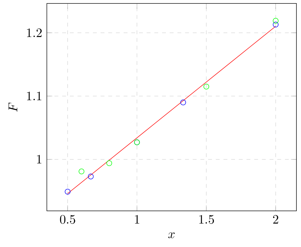
The result is
Which is in error at by about 3%.
If you are thinking that this looks like a quadratic fit might be better, you are correct, but there really isn’t time to do that for this experiment.
Marking scheme:
| Data | vary | 0.10 pts |
|---|---|---|
| vary | 0.10 pts | |
| cm | 0.05 pts | |
| cm | 0.05 pts | |
| V | 0.05 pts | |
| table has units | 0.05 pts | |
| cm | 0.05 pts | |
| cm | 0.05 pts | |
| well distributed | 0.05 pts | |
| 0.05 pts | ||
| Correct calculations of derived quantities | 0.10 pts | |
| 10 or more points | 0.30/0.30 | |
| 9 points | 0.25/0.30 | |
| 8 points | 0.20/0.30 | |
| 6 or 7 points | 0.10/0.30 | |
| 5 or fewer points | 0.05/0.30 | |
| Plotting | covers % of area | 0.10 pts |
| Axis labels | 0.05 pts | |
| Axis units correct | 0.05 pts | |
| one plotting mistake | -0.05/-0.10 | |
| two or more plotting mistakes | -0.10/-0.10 | |
| Fit | line drawn on graph | 0.10 pts |
| slope correctly computed with units | 0.10 pts | |
| 0.10 pts | ||
| sum | 1.5 pts |
Оригинал в Архива: exam-experiment-Q2-english.pdf · официални решения: experiment_solutions (1).pdf