IPhO 2023 — Задача 1. Characterization of Soil Colloids (10 points)

Theory — Q1-1, English (Official): Characterization of Soil Colloids (10 points) — International Physics Olympiad 2023 Tokyo Japan · 10 т.

Условие

Colloidal science is useful to characterize soil particles because many of them can be regarded as colloidal particles of micrometer size. For example, Brownian motion (random motion of colloidal particles) can be used to measure particle sizes.

Part A. Motions of colloidal particles (1.6 points)

We analyze the one-dimensional Brownian motion of a colloidal particle with mass $M$. The equation of motion for its velocity $v(t)$ reads:

$M\dot{v} = -\gamma v(t) + F(t) + F_{\mathrm{ext}}(t), \qquad (1)$

where $\gamma$ is the friction coefficient, $F(t)$ is a force due to random collisions with water molecules, and $F_{\mathrm{ext}}(t)$ is an external force. In Part A, we assume $F_{\mathrm{ext}}(t) = 0$.

In the following, you may use $\tau$ in your answers.

Part B. Effective equation of motion (1.8 points)

Results so far imply that particle velocities $v(t)$ and $v(t')$ may be regarded as uncorrelated random quantities if $|t - t'| \gg \tau$. On this basis, we introduce a theoretical model to approximately describe the one-dimensional Brownian motion, where the velocity changes randomly at each time interval $\delta\ (\gg \tau)$, i.e.,

$v(t) = v_n \quad (t_{n-1} < t \leq t_n), \qquad (2)$

with $t_n = n\delta\ (n = 0, 1, 2, \cdots)$ and a random quantity $v_n$. It satisfies

$\langle v_n \rangle = 0, \quad \langle v_n v_m \rangle = \begin{cases} C & (n = m), \\ 0 & (n \neq m), \end{cases} \qquad (3)$

with a parameter $C$ depending on $\delta$. Here $\langle X \rangle$ indicates the expectation value of $X$. That is, if you draw random numbers $X$ infinite times, the mean will be $\langle X \rangle$.

Now we consider the particle displacement $\Delta x(t) = x(t) - x(0)$ for $t = N\delta$ with an integer $N$.

Part C. Electrophoresis (2.7 points)

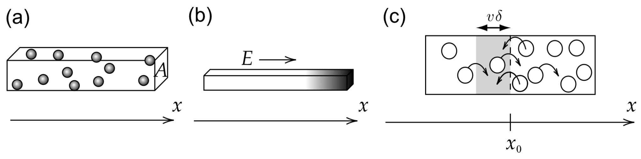
Here we discuss electrophoresis, i.e., transport of charged particles by an electric field. Suspension of colloidal particles with mass $M$ and charge $Q\ (> 0)$ is put in a narrow channel with a cross-section $A$ (Fig.1(a)). We ignore the interaction between particles, effects of the wall, the fluid, the ions therein, and gravity.

By applying a uniform electric field $E$ in the $x$-direction, particles are transported and their concentration $n(x)$ (particle number per unit volume) becomes non-uniform (Fig.1(b)). When $E$ is removed, this non-uniformity gradually disappears. This is due to Brownian motion of particles. If $n(x)$ is not uniform, the numbers of right-going and left-going particles may differ (Fig.1(c)). This generates a particle flux $J_D(x)$, the mean number of particles flowing at $x$ along the $x$-axis per unit cross-sectional area and unit time. This flux is known to satisfy

$J_D(x) = -D\,\frac{dn}{dx}(x), \qquad (4)$

where $D$ is called the diffusion coefficient.

Now let's assume, for simplicity, that half of the particles have velocity $+v$ and the other half have velocity $-v$. Let $N_+(x_0)$ be the number of particles with velocity $+v$ that cross $x_0$ from left to right per unit cross-sectional area and unit time. For particles with velocity $+v$ to cross $x_0$ in the time interval $\delta$, they should be in the shaded region of Fig.1(c). Since $\delta$ is small, we have $n(x) \simeq n(x_0) + (x - x_0)\frac{dn}{dx}(x_0)$ in this region.

We define $N_-(x_0)$ as the counterpart of $N_+(x_0)$ for the velocity $-v$. With this, we have $J_D(x_0) = \langle N_+(x_0) - N_-(x_0) \rangle$. According to Eq.(3), we have $\langle v^2 \rangle = C$.

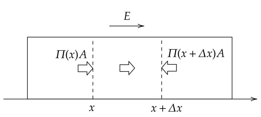
Now we discuss the effect of osmotic pressure $\Pi$. It is given by $\Pi = \frac{n}{N_A}RT = nkT$ with the Avogadro constant $N_A$, the gas constant $R$, temperature $T$, and the Boltzmann constant $k = \frac{R}{N_A}$. Let us consider the non-uniform concentration formed under the electric field $E$ (Fig.1(b)). Since $n(x)$ depends on $x$, so does $\Pi(x)$. Then the forces due to $\Pi(x)$ and $\Pi(x+\Delta x)$ must be balanced with the total force from the field $E$ acting on the particles (Fig.2). Here we consider small $\Delta x$, so that $n(x)$ can be regarded as constant over this range, while $n(x+\Delta x) - n(x) \simeq \Delta x\,\frac{dn}{dx}(x)$.

Let us discuss the balance of the flux now. Besides the flux $J_D(x)$ due to the Brownian motion, there is also a flux due to the electric field, $J_Q(x)$. It is given by

$J_Q(x) = n(x)u, \qquad (5)$

where $u$ is the terminal velocity of particles driven by the field.

Part D. Mean square displacement (2.4 points)

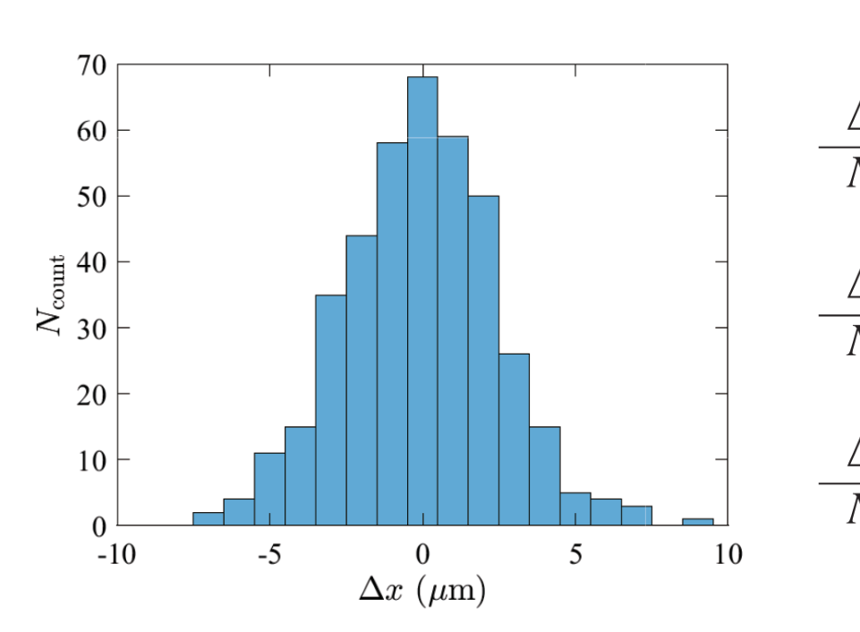
Suppose we observed the Brownian motion of an isolated, spherical colloidal particle with radius $a = 5.0\ \mu\mathrm{m}$ in water. Figure 3 shows the histogram of displacements $\Delta x$ measured in the $x$-direction at every interval $\Delta t = 60\ \mathrm{s}$. The friction coefficient is given by $\gamma = 6\pi a\eta$ with water viscosity $\eta = 8.9 \times 10^{-4}\ \mathrm{Pa \cdot s}$ and the temperature was $T = 25\ {}^{\circ}\mathrm{C}$.

$\Delta x\ (\mu\mathrm{m})$	$-10$	$-9$	$-8$	$-7$	$-6$	$-5$	$-4$
$N_{\mathrm{count}}$	0	0	0	2	4	11	15

$\Delta x\ (\mu\mathrm{m})$	$-3$	$-2$	$-1$	$0$	$1$	$2$	$3$
$N_{\mathrm{count}}$	35	44	58	68	59	50	26

$\Delta x\ (\mu\mathrm{m})$	$4$	$5$	$6$	$7$	$8$	$9$	$10$
$N_{\mathrm{count}}$	15	5	4	3	0	1	0

Now we extend the model in Part B to describe the motion of a particle with charge $Q$ under an electric field $E$. The particle velocity $v(t)$ considered in Eq.(2) should be replaced by $v(t) = u + v_n\ (t_{n-1} < t \leq t_n)$ with $v_n$ satisfying Eq. (3) and $u$ being the terminal velocity considered in Eq.(5).

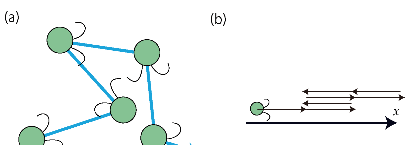
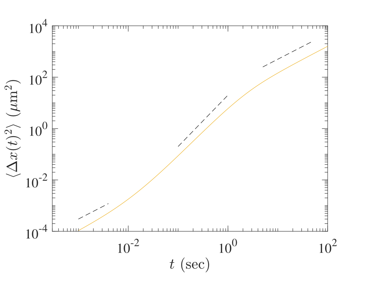
Next, we consider swimming microbes (Fig.4(a)), in one dimension for simplicity (Fig.4(b)). These are spherical particles with radius $a$. They swim at velocity either $+u_0$ or $-u_0$, the sign chosen randomly at every time interval $\delta_0$ without correlation. The observed motion is a combination of displacements due to swimming and those due to the Brownian motion of a spherical particle.

Part E. Water purification (1.5 points)

Here we discuss the purification of water including colloid-like soil particles, by adding electrolytes to coagulate them. Particles interact through van der Waals force and electrostatic force, the latter including effects of both surface charges and the surrounding layer of oppositely charged ions (such ions and their layer are called counter-ions and the electric double layer, respectively; see Fig.6(a)). As a result, the interaction potential for particle distance $d$ (Fig.6(b)) is given by

$U(d) = -\frac{A}{d} + \frac{B\epsilon(kT)^2}{q^2}e^{-d/\lambda}, \qquad (6)$

where $A$ and $B$ are positive constants, $\epsilon$ is the dielectric constant of water, and $\lambda$ is the thickness of the electric double layer. Assuming that charges of ions are $\pm q$, we have

$\lambda = \sqrt{\frac{\epsilon kT}{2N_A q^2 e}}, \qquad (7)$

where $e$ is the molar concentration of ion.

A.1 Consider that a water molecule collides with the particle at $t = t_0$, giving impulse $I_0$, and $F(t) = 0$ afterward. If $v(t) = 0$ before the collision, $v(t) = v_0 e^{-(t-t_0)/\tau}$ for $t > t_0$. Determine $v_0$ and $\tau$, using $I_0$ and necessary parameters in Eq.(1). [0,8 т.]

A.2 Actually, water molecules collide with the particle one after another. Suppose the $i$th collision gives the impulse $I_i$ at time $t_i$ and determine $v(t)$ on condition that $t > 0$ and $v(0) = 0$. Also give the inequality specifying the range of $t_i$ that needs to be considered for a given $t$. In the answer sheet, it is not necessary to specify this range in the expression for $v(t)$. [0,8 т.]

B.1 Determine $\langle \Delta x(t) \rangle$ and $\langle \Delta x(t)^2 \rangle$ using $C$, $\delta$, and $t$. [1 т.]

B.2 The quantity $\langle \Delta x(t)^2 \rangle$ is called the mean square displacement (MSD). It is a characteristic observable of the Brownian motion, which corresponds to the limiting case $\delta \to 0$. From this, we can show $C \propto \delta^{\alpha}$ and $\langle \Delta x(t)^2 \rangle \propto t^{\beta}$. Determine the values of $\alpha$ and $\beta$. [0,8 т.]

C.1 Express $N_+(x_0)$ using necessary quantities from $v$, $\delta$, $n(x_0)$, and $\frac{dn}{dx}(x_0)$. [0,5 т.]

C.2 Determine $J_D(x_0)$ using necessary quantities from $C$, $\delta$, $n(x_0)$, and $\frac{dn}{dx}(x_0)$. Using this and Eq.(4), express $D$ in terms of $C$ and $\delta$, and $\langle \Delta x(t)^2 \rangle$ in terms of $D$ and $t$. [0,7 т.]

C.3 Express $\frac{dn}{dx}(x)$ using $n(x)$, $T$, $Q$, $E$, and $k$. [0,5 т.]

C.4 To determine $u$, we use Eq.(1) with $F_{\mathrm{ext}}(t) = QE$. Since $v(t)$ is fluctuating, we consider $\langle v(t) \rangle$. Assuming $\langle v(0) \rangle = 0$ and using $\langle F(t) \rangle = 0$, evaluate $\langle v(t) \rangle$ and obtain $u = \lim_{t \to \infty} \langle v(t) \rangle$. [0,5 т.]

C.5 The flux balance reads $J_D(x) + J_Q(x) = 0$. Express the diffusion coefficient $D$ in terms of $k$, $\gamma$, and $T$. [0,5 т.]

D.1 Estimate the value of $N_A$ without using the fact that it is the Avogadro constant, up to two significant digits from the data in Fig.3. The gas constant is $R = 8.31\ \mathrm{J/K \cdot mol}$. Do not use the value of the Boltzmann constant $k$ given in General Instructions. As for the Avogadro constant, you might obtain a value different from that in General Instructions. [1 т.]

D.2 Express the MSD $\langle \Delta x(t)^2 \rangle$ in terms of $u$, $D$, and $t$. Obtain approximate power laws for small $t$ and large $t$, as well as the characteristic time $t_*$ where this change occurs. Draw a rough graph of MSD in a log-log plot, indicating the approximate location of $t_*.$ [0,8 т.]

D.3 Figure 5 displays the MSD $\langle \Delta x(t)^2 \rangle$ of those microbes, showing different power laws for small, large, and intermediate $t$, as indicated by dashed lines. Obtain the power law for each time range and express it using necessary quantities from $D$, $u_0$, $\delta_0$, and $t$. [0,6 т.]

E.1 Addition of sodium chloride (NaCl) to the suspension causes colloidal particles to coagulate. Determine the lowest concentration $c$ of NaCl necessary for coagulation. It is sufficient to consider two particles without thermal fluctuations, i.e., $F(t) = 0$ in Eq.(1), and assume that the terminal velocity for the given potential force is reached instantaneously. [1,5 т.]

Решение

---

Оригинал в Архива: IPhO_2023_Q1.pdf · официални решения: IPhO_2023_S1.pdf