IPhO 2024, experiment — Задача 1. Heat Conduction in a Copper Rod (10 points)

Heat Conduction in a Copper Rod (10 points) · 10 т.

Условие

The Experimental Setup

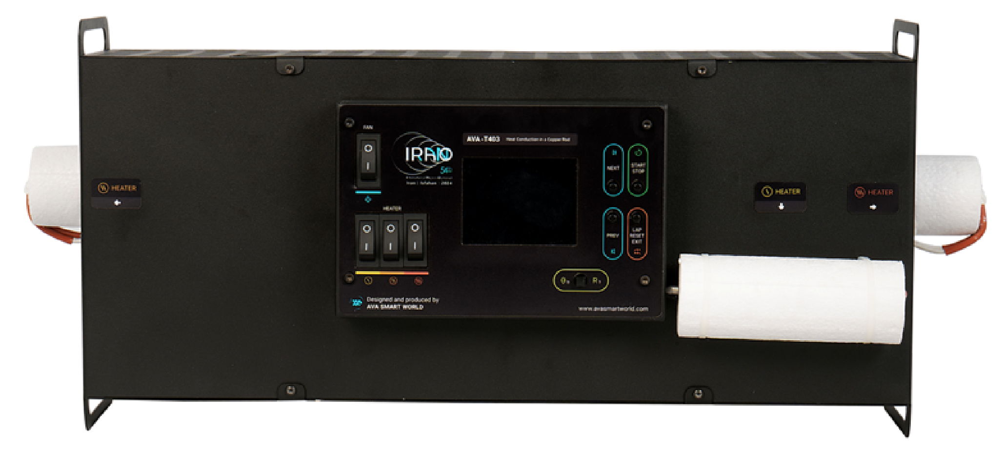
In this experiment a 57.0 cm long copper rod with a diameter of 1.20 cm has been placed across the length of a metal box which is supported by square flanges (Figure 1). The metal box serves to isolate the airflow inside the box.

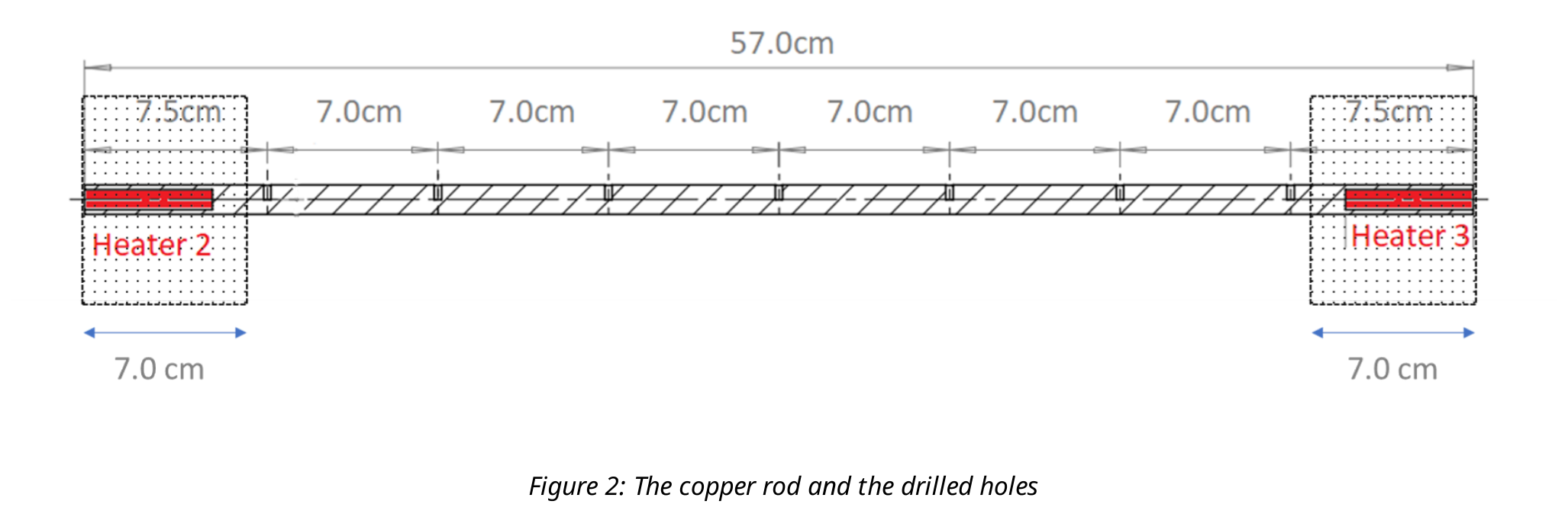
As shown in Figure 2, 7.0 cm from eachside of the two ends of the rod is insulated by styrofoam. Seven holes have been drilled in the rod at equal distances of 7.0 cm; each hole has a depth of 0.6 cm and a temperature sensor (a thermistor) has been placed inside each drilled hole. These sensors have been numbered 1 through 7, from left to right. A similar sensor, numbered 8, has been placed within the box to monitor the ambient temperature of the box ($\theta_{\mathrm{b}}$).

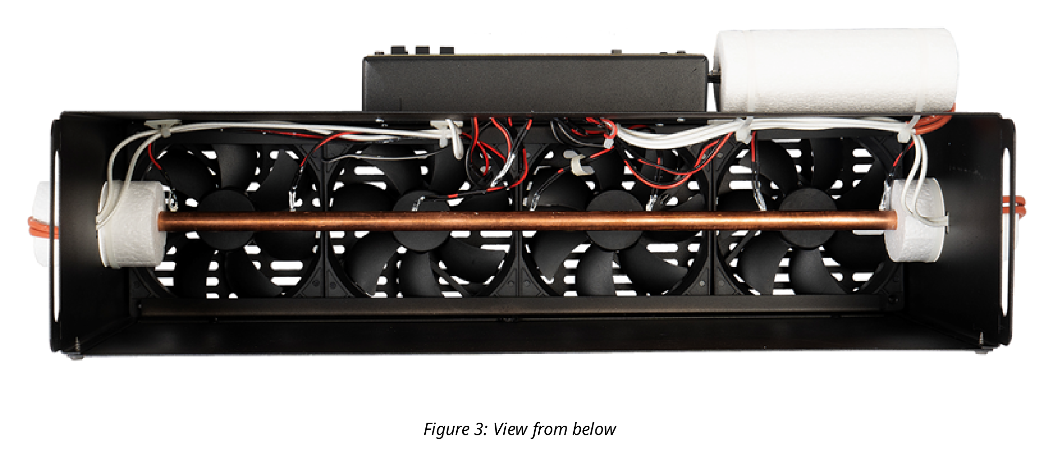
At the two insulated ends of the rod, two electric heaters with different output powers have been installed inside 5.2 cm-long holes, drilled longitudinally. The left and right heaters are designated as Heaters nos. 2 and 3, respectively. Four fans at the top of the metal box, control the air flow within the box and around the rod. These fans, as well as the copper rod, can be seen from below as shown in Figure 3.

A control panel, which we call AVA-T403, has been installed on the front. All the switches for turning on the various components of the experiment: the fans, the heaters, the timer, etc. are on this panel and all the measurements made by the sensors are displayed on its monitor. The power necessary to run all the instruments is provided by a 24 V power supply when connected to the power outlet. It lies next to the box.

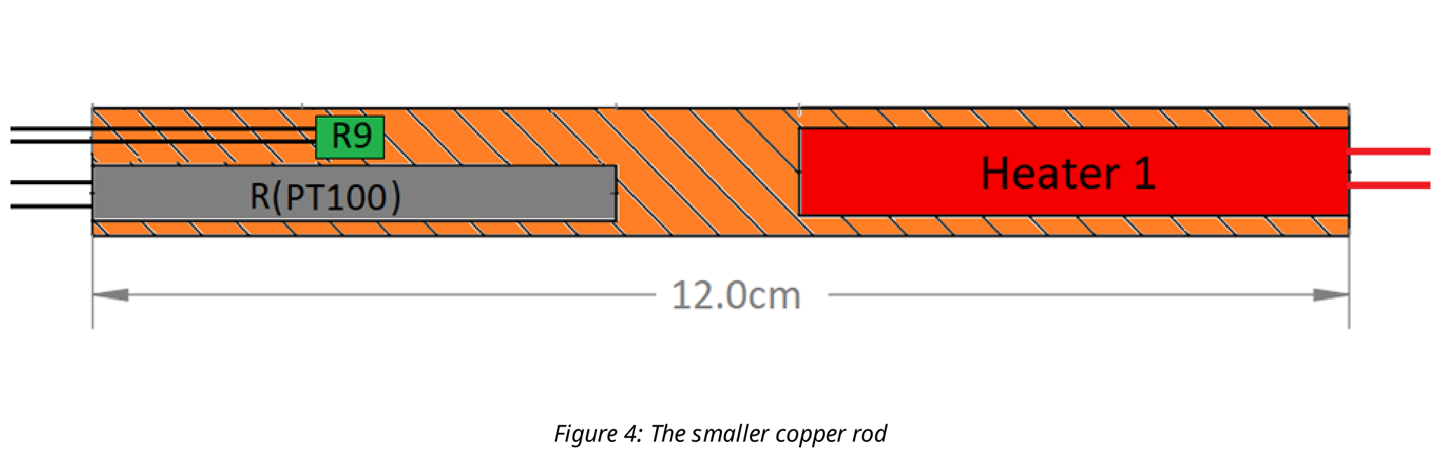
To the right of the control panel, a smaller 12.0 cm copper rod is installed; it is also covered with styrofoam. Under the styrofoam, Heater no. 1 with an output power of $1.95 \pm 0.06\ \mathrm{W}$ has been inserted inside a longitudinal hole at the right as shown in Figure 4. At the other end, another longitudinal hole has been drilled in which an PT100 (Platinum Thermometer 100) thermistor bundled together with another thermistor ($R_9$) (similar to the other thermistors) have been inserted. These two sensors and the heater are connected to AVA, and AVA indicates the values of their resistance (in $\Omega$).

Please observe the following points:

1. Do not touch and activate the buttons on the equipment before it is asked you to do so.
2. You do not need to do anything regarding the setup. Take care not to disturb the setup and not to disconnect any wires.
3. Don't move the setup during the experiment.
4. If the message "Turn off Heater1" appears on the monitor, immediately turn off Heater no. 1.
5. Turning on the heaters will increase the temperature, so it will take extra time for the system to reach its steady state, make sure that you do not turn on a heater unnecessarily.
6. Errors need to be calculated and reported whenever the $\pm$ sign is present in the answer sheet.
7. Regression, (denoted by reg in the formula below and shown as r on the calculator), is a number between 1 and -1 showing how much the data can be fitted to a line. If $|\mathrm{reg}| = 1$ it means that the data are completely on a line.

We can use the following formula to calculate the uncertainty of the slope b :

$\Delta b = b\sqrt{\frac{1}{(n-2)}\left(\frac{1}{\mathrm{reg}^2} - 1\right)}$

in which $n$ is the number of data points.

The Equipment

1. Generally, Electrical resistors have different behaviors in response to a change in temperature. One of the widely used resistors is PT100 which has a linear behavior over a considerable range of temperatures, i.e.

$R = R_0(1 + \alpha\theta) \quad (1)$

in which $R_0$ is the value of the resistance at the $0^{\circ}\,\mathrm{C}$, $\alpha$ is a constant coefficient (within the range of temperatures for this problem), and $\theta$ is the temperature in degrees Celsius. The value of $\alpha$ for the resistor used in this problem is $0.0039083\ {}^{\circ}\mathrm{C}^{-1}$. For PT100, $R_0 = 100.00\ \Omega$.

2. The thermistors 1 through 9 have a nonlinear behavior in response to changes in temperature, and are usually used for measuring small changes in temperature. The resistance of these thermistors changes with temperature as follows:

$R' = R'_0\,\mathrm{e}^{\frac{E_{\mathrm{g}}}{2k_{\mathrm{B}}T}} \quad (2)$

Where $R_0'$ is a constant, $k_{\mathrm{B}} = 8.61733 \times 10^{-5}\ \mathrm{eV/K}$ is the Boltzmann constant, $T$ is the temperature in kelvins and $E_{\mathrm{g}}$ is the energy gap for the thermistor's semiconductor material. Remember that $T = (\theta + 273.15)\ \mathrm{K}$

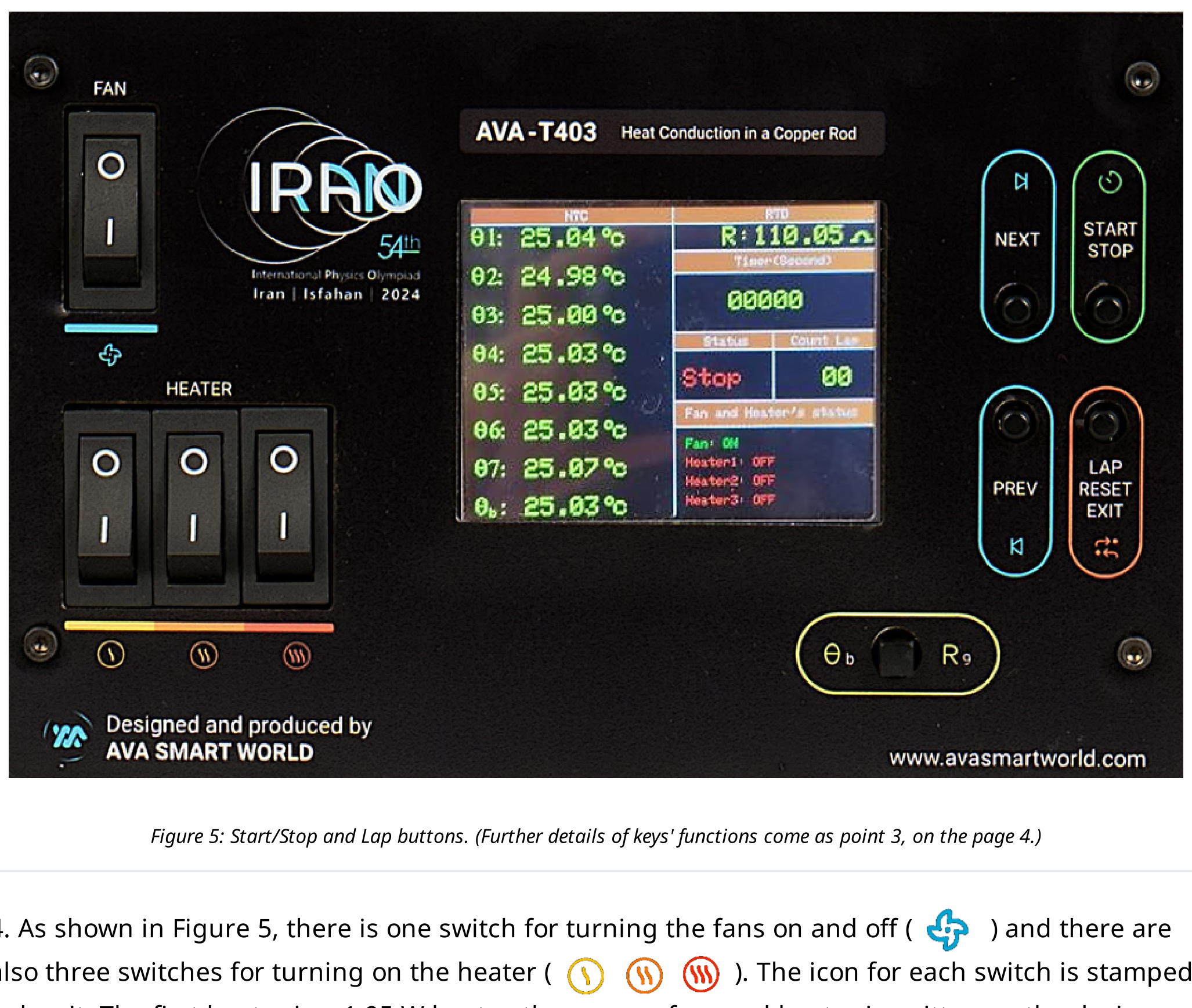
3. The digital device AVA was designed by Iranian engineers specifically for this experiment. AVA measures the instantaneous resistances of Thermistors 1 through 7, PT100, and $\theta_{\mathrm{b}}$ or $R_9$. every two seconds. Then, based on the formula 2, reports the temperature of these sensors. However, for Sensor no. 9, only the value of the resistance is displayed. On the left of AVA's monitor, the temperatures of sensors 1 through 7 are displayed in a column. The last row, however, only shows at each instance, either the temperature of sensor 8, or the resistance of Sensor 9 ($R_9$). You can toggle between these two values by pressing the $\theta_{\mathrm{b}} - R_9$ button shown in Figure 5.

AVA also has a timer, which works very much like any commercial timer: by pressing the Start/Stop button, the timer starts measuring the time elapsed, and pressing the Start/Stop button again stops the timer. While the timer is working, pressing the Lap button will result in all the displayable values being saved. Pressing the same button when the timer is not working resets the timer, however, the saved data will not be erased. To erase the data the Lap/Reset button has to pressed and held for 5 seconds.

The saved data can be seen by repeatedly pressing the Next/Prev button: pressing Prev shows older data, pressing Next shows newer data. All saved data will be erased in case the device is switched off and on. The device will not turn off automatically.

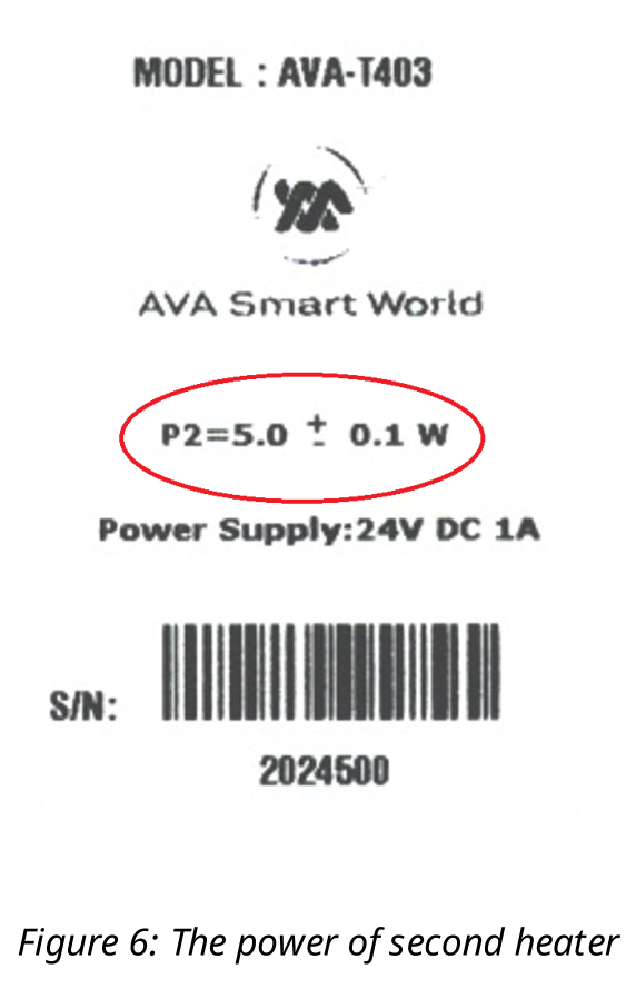
4. As shown in Figure 5, there is one switch for turning the fans on and off ( $\approx$ ) and there are also three switches for turning on the heater ( $\,\wr\,$ $\,\wr\!\wr\,$ $\,\wr\!\wr\!\wr\,$ ). The icon for each switch is stamped below it. The first heater is a 1.95 W heater, the power of second heater is written on the device as shown in Figure 6, and the power of third heater is unknown.

Theory

In this problem, heat is transferred inside the rod through conduction, and transferred from the rod to the surrounding air through natural or forced convection. Also, due to the heat capacity of the rod, some of the heat injected into the rod is used up to raise the temperature of the rod.

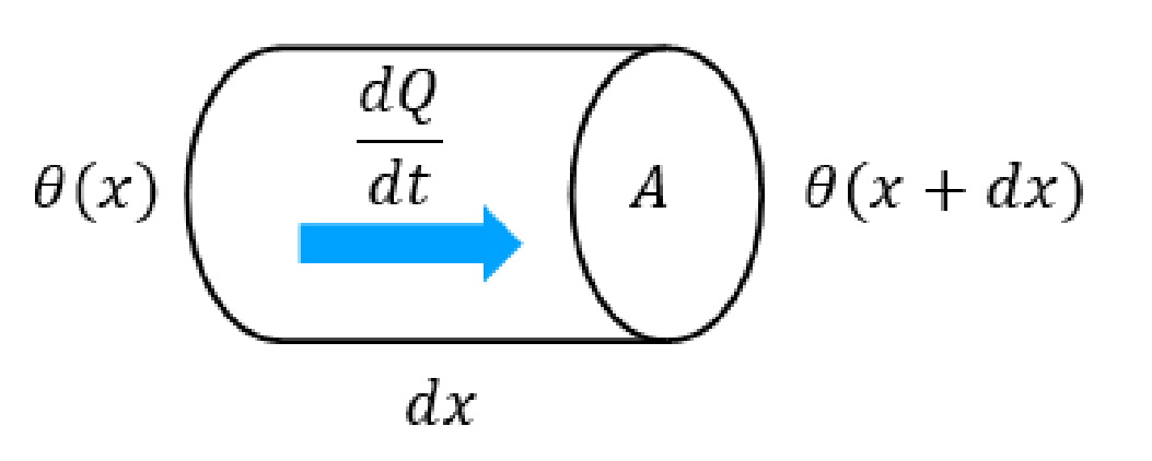
(a) Heat conduction: for a heat conductor in the shape of a rod with no heat loss from its lateral surface, the rate of heat transfer, ${}^{dQ}/_{dt}$, through a differential element (Figure 7) at the steady state is as follows

$\frac{dQ}{dt} = -kA\,\frac{d\theta}{dx} \quad (3)$

where $d\theta$ is the temperature difference between the two edges of the differential element, $A$ is the cross-sectional area, $dx$ is the length of the differential element, and k is the heat transfer coefficient (heat conductivity) which depends on the type of material the rod is made of.

(b) Convection: For any object exchanging heat with the air through its lateral surface, the following relationship holds:

$\frac{dQ}{dt} = -hS\Delta\theta \quad (4)$

in which $S$ is the area of the lateral surface, $\Delta\theta$ is the temperature difference between the object and the surrounding air, and $h$ is the convective heat transfer coefficient which is a function of the shape of the object and the nature of the heat flow through the sides of the object.

The Experiment:

In order to save time, we recommend that you turn on Heater 2 and the fans which are needed in Part B. Make sure that the other heaters are not turned on.

Part A: The short copper rod (3.9 points)

A-0 Write numbers 0 to 9 in the table. (0 pt)

Before turning on Heater 1, the small rod is at the same temperature as its environment. Tasks A-1 to A-3 are related to the heating process and tasks A-4 to A-7 correspond to the cooling process of the rod.

A-1 (0.2 pt) Record the initial value of resistance $R_{\mathrm{env}}$ (resistance of PT100) when it is at the temperature of its environment. Using Eq.1, find this temperature.

Let us denote the total heat capacity of the rod and the heater and the sensors by $C_{\mathrm{S}}$. To find $C_{\mathrm{S}}$ we should turn on Heater 1 and measure the change in the value of resistance for at least 150 seconds. Note that there is a time delay in the heating and cooling of the sensors.

A-2 (0.5 pt) In time intervals of approximately 10 seconds record the value of $R$. Do this at least 15 times.

A-3 (0.8 pt) Draw a diagram for Part A-2, fit a line to your data and find its slope. Using the slope find $C_{\mathrm{S}}$.

Wait until the value of $R$ reaches $120\ \Omega$ and then turn off Heater 1. The temperature of the rod and the resistance $R$ will start to decrease slowly after a few seconds. When PT100 is cooling down, the resistance is given by:

$R - R_{\mathrm{env}} = Ae^{-\gamma t} \quad (5)$

in which $A$ and $\gamma$ are constants.

A-4 (0.5 pt) At several different instances of time, measure the value of $R - R_{\mathrm{env}}$.

A-5 (0.7 pt) Make a semi-logarithmic plot of your data in part A-4. Then find $\gamma$.

The insulator around the rod causes the resistors to reach thermal equilibrium sooner, and, the rod to have a more uniform temperature profile.

A-6 (0.5 pt) Measure and record the resistance $R_9$ of Thermistor 9 in terms of $R$. Measure at least seven different values of $R$, preferably in the $114 - 120\ \Omega$ range.

A-7 (0.7 pt) Draw a diagram of the resistance $R_9$ versus $1/T$ on the given semi-logarithmic graph and find the magnitude of the energy gap $E_{\mathrm{g}}$ in units of eV.

Part B: The long copper rod (4.1 points)

Wait for the rod to reach a steady state i.e. the measured temperatures at all points remain constant, and then answer the following questions. We shall denote the temperatures of Thermistors 1-7 by $\theta_1$ through $\theta_7$ respectively. The location of Thermistor 1 corresponds to $x = 0$.

B-1 (0.4 pt) When the rod reaches steady state, measure and record the temperature $\theta_{\mathrm{b}}$ and $\theta_x$ for the seven points on the rod.

In order to save time, take a look at Part C and then continue Part B.

B-2 (0.4 pt) On semi-log paper, draw a diagram for the difference between the temperature of the box and the temperature at point $x$, $(\theta_x - \theta_{\mathrm{b}})$ along the length of the rod.

It can be shown that as a function of the distance from Heater 2 along the length of the line, the temperature obeys the following relation:

$\theta_x = \theta_{\mathrm{b}} + Ae^{-\lambda x} + Be^{\lambda x} \quad (6)$

in which $\theta_{\mathrm{b}}$ the ambient temperature of the box, $A$ and $B$ are constants, and $\lambda = \sqrt{\frac{2h}{kr}}$ where $r$ is the radius of the rod. As a first step, we can ignore the data corresponding to large values of $x$ and take $B$ to be zero. In this case we can find $\lambda$ and $A$ to a first approximation, let us call them $\lambda^{(0)}$ and $A^{(0)}$:

B-3 (0.6 pt) Use the temperatures $\theta_1$ through $\theta_5$ and find $\lambda^{(0)}$ and $A^{(0)}$ using the diagram of Part B-2.

The temperature at the end of the rod farthest from the heater does not change with $x$. Assume this happens around a distance $x = d$. One can use this to determine $B$ in terms of $\lambda$, $A$, and $d$:

B-4 (0.4 pt) Express $B$ in terms of $\lambda$, $A$, and $d$, and for $d = 44.0$ cm. Find its numerical value using the results of Part B-3. Denote this quantity as $B^{(1)}$.

Now we can use the value obtained for $B$ to correct the previous calculation. To do so, assume:

$\theta'_x = \theta_x - B^{(1)}e^{\lambda^{(0)}x}$

B-5 (0.4 pt) Find $\theta_1'$ through $\theta_7'$ and complete the columns added to table B-1.

B-6 (1.0 pt) Draw a new diagram to obtain the values for $\lambda$ and $A$ Denote them by $\lambda^{(1)}$ and $A^{(1)}$ respectively.

To obtain accurate approximations, the corrections should be repeated many times, but in the end, we'll find that the final answer is close to $\lambda = \frac{\lambda^{(0)}+\lambda^{(1)}}{2}$ and $A = \frac{A^{(0)}+A^{(1)}}{2}$.

B-7 (0.9 pt) By balancing the input and output powers of the copper rod, find $h$ and $k$.

Part C: Measuring the unknown power (2.0 points)

While the fans are on, turn on Heaters 2 and 3, and wait until the temperature reaches equilibrium at all points of the copper rod. (This will take about 15 minutes.)

C-1 (0.4 pt) Measure and record the temperatures $\theta_1$ through $\theta_7$.

It can be shown that, in this case, the temperature in terms of $x$ varies as follows

$\theta_x - \theta_{\mathrm{b}} = A'\cosh(\lambda(x - x_0))$

in which $A'$ is a constant and $\cos h(u)$ is the hyperbolic cosine function of u defined as:

$\cos h\left(u\right) = \frac{e^u + e^{-u}}{2}$

C-2 (0.6 pt) Draw the diagram of temperature versus distance and find $x_0$.

C-3 (1.0 pt) Using your own method to find the effective power of Heater 3. Explain your method as clearly as possible by writing down explicitly the mathematical formulas you have used to arrive at your results.

Решение

Оригинал в Архива: IPhO_2024_Q4.pdf · официални решения: IPhO_2024_S5.pdf