Съдържание

Условие Part A. Theoretical principles of ellipsometry Part B. Kinetics of oxidation Отговори Решение

ISPhO 2024, Теория — Задача 1. T1. Thermal oxidation

Оригинал на условието (PDF)Съобщи за грешка

Всички материали от ISPhO 2024

ISPhO, July, 2024 — T1. Thermal oxidation

Условие

Thermal oxidation is the process of creating a very thin (tens/hundreds of nanometres) film of silicon dioxide $\mathrm{SiO_2}$ on the surface of silicon Si at high temperatures. This technology is an essential part of the manufacturing process of integrated circuits and MOSFETs (metal-oxide-semiconductor), which form the basis of modern electronics. If you place silicon Si in an aerobic environment, the oxidation process of $\mathrm{Si} + \mathrm{O_2} \to \mathrm{SiO_2}$ will begin. For the description of crystalline silicon and flat oxide films of sufficient thickness (starting from ten nanometres), the Dill-Grove model (1965) does well, but a detailed description of the growth mechanism in other conditions is still an unsolved scientific problem.

Silicon is opaque to visible light, while its dioxide is transparent. These optical properties, combined with the fact that the dioxide film has a thickness of tens of nanometres, create ideal conditions for very precise optical control of the thickness of the $\mathrm{SiO_2}$ layer.

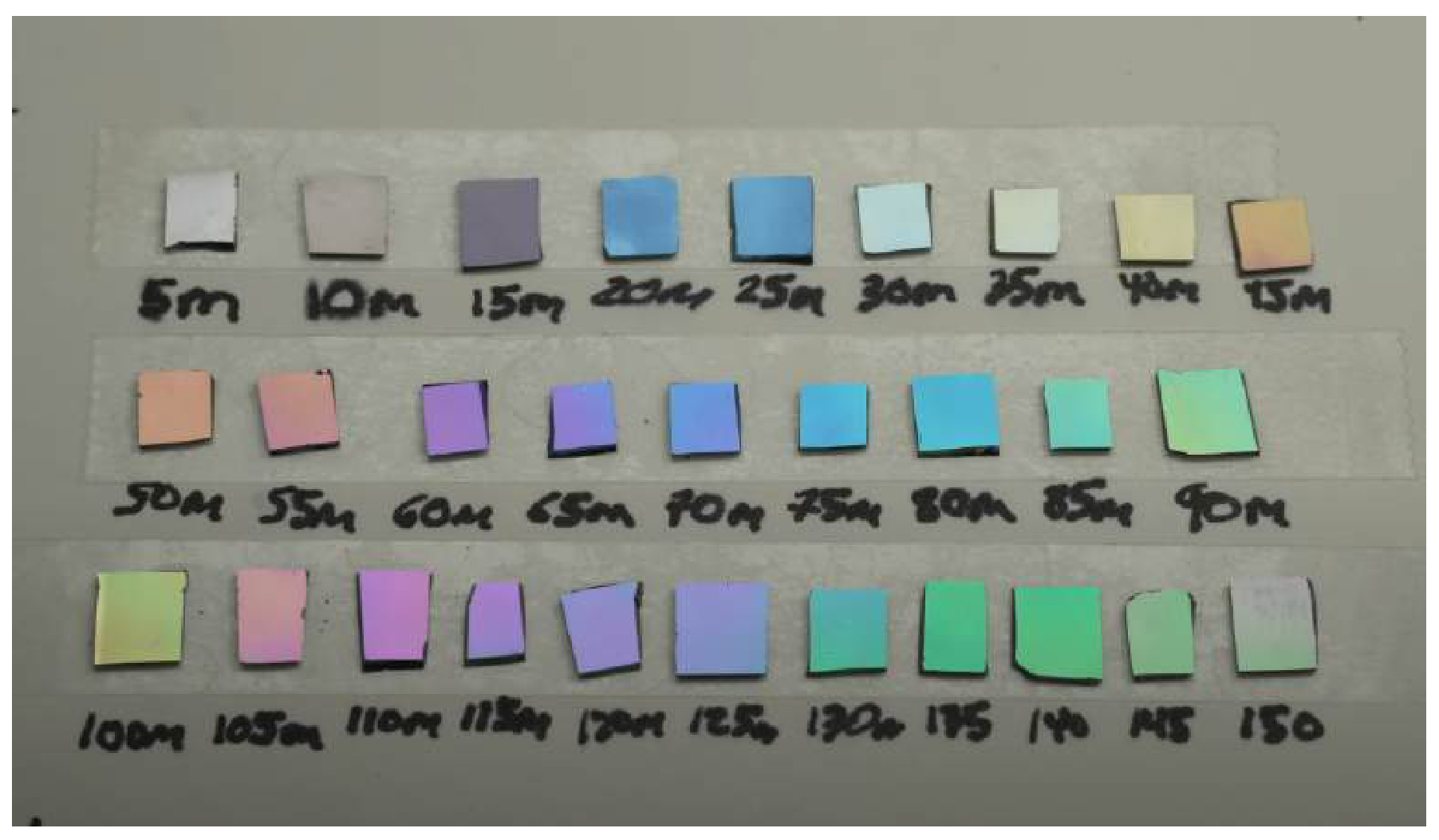
Photograph of three rows of small oxidized silicon squares on tape, each labelled by hand with the oxidation time from 5m to 150; the colours change from grey through purple, blue, yellow, pink and green. — The change in the visible color of the silicon substrate at different oxidation times. ”Growing Colorful Oxide Layers on Silicon” by ProjectsInFlight on YouTube.

We will investigate the film growth by using ellipsometry, a powerful technique for studying the optical properties of thin films. It is based on a comparison of the amplitude coefficients of reflection of $s$ -polarized and $p$ -polarized waves (from the German ”senkrecht” – perpendicular, ”parallel” – parallel) from the surface of the film. The measurement results are represented by ellipsometric angles $\Psi$ , $\Delta$ :

\frac{r_p}{r_s} = \tan\Psi \cdot e^{i\Delta},

where the value of $\Psi$ corresponds to the ratio of amplitudes upon reflection of $p$ - and $s$ -polarized waves, and the value of $\Delta$ corresponds to the phase difference between them.

Ellipsometry measures precisely the relative difference between waves (ratio of amplitudes and phase difference) with different polarizations, so it is very resistant to various fluctuations in the power of the radiation source and the sensitivity of the receiver. Ellipsometry also makes it possible to measure the characteristics of a sample without direct mechanical contact with it, which allows measurements to be carried out in real time and in situ (from lat. – ”on the spot”, directly).

During the entire task, the wavelength of the incident wave is marked as $\lambda$ . In the optical range, substances do not have significant magnetic qualities, therefore, all materials under consideration have $\mu = 1$ .

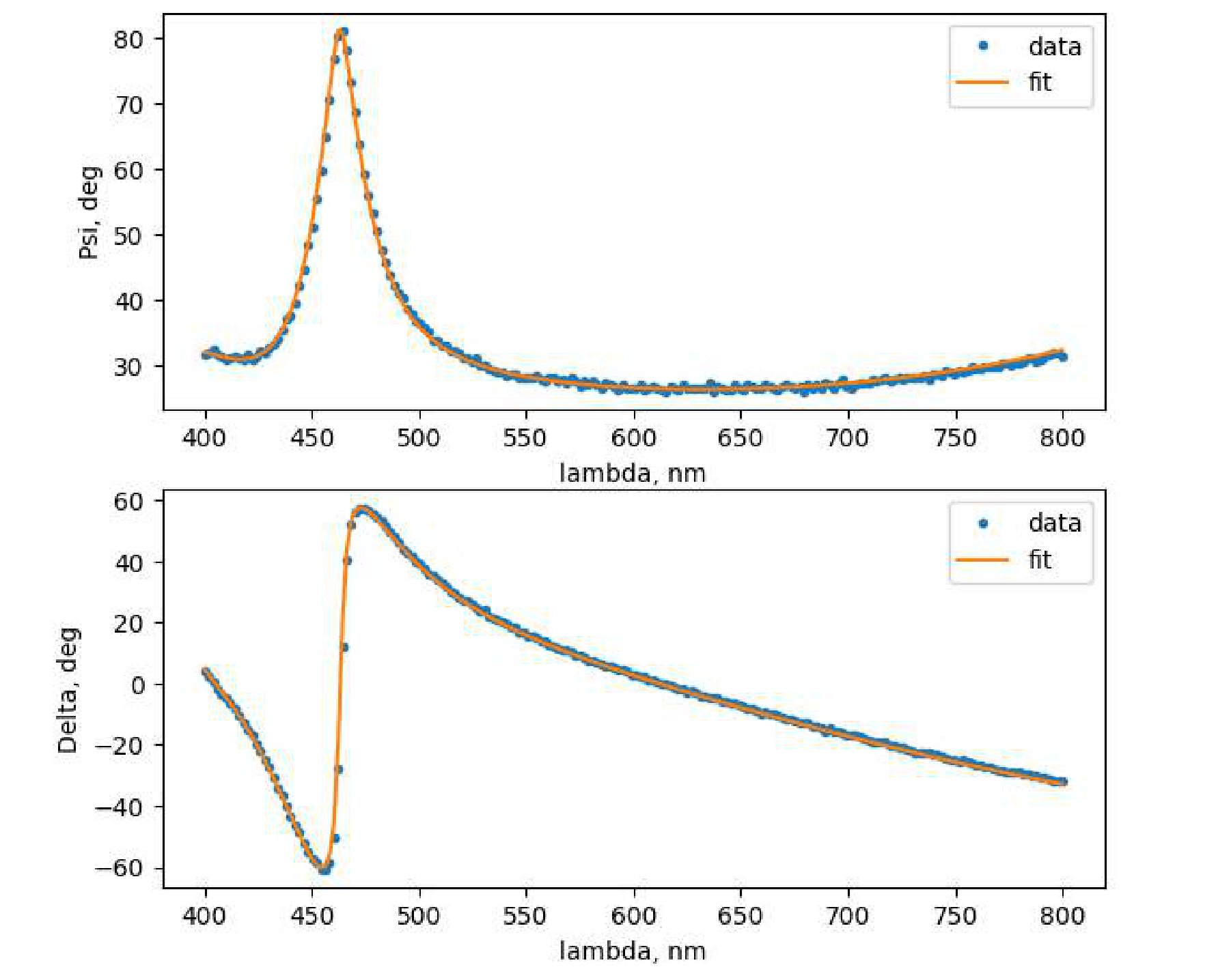
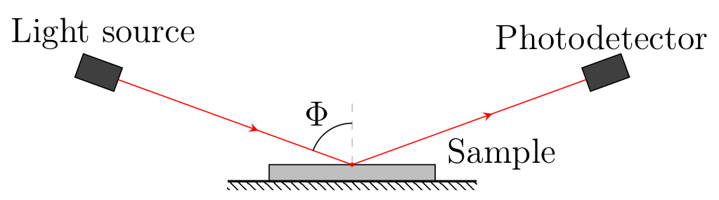
Two stacked plots against lambda, nm from 400 to 800: the upper one Psi, deg (about 30 to 80, sharp peak near 460 nm), the lower one Delta, deg (from -60 to 60, dip near 455 nm then a jump and slow decrease); data points and fit curve with a legend data/fit. — Example of an ellipsometric spectrum $\Psi, \Delta$

Scheme: a light source on the left sends a ray at angle Phi to the normal onto a sample on a hatched base; the reflected ray goes to a photodetector on the right. Labels: Light source, Photodetector, Sample, Φ. — Optical scheme of the ellipsometer: a light source, a Photodetector, and a test sample.

Attention! Place the files you want to attach to the report in the “report” folder.

Attention! It is enough to make only A7 to moving on to part B.

Part A. Theoretical principles of ellipsometry

Maxwell’s equations in a non-magnetic dielectric have the form

\operatorname{div}\vec{D} = 0 \qquad \operatorname{rot}\vec{E} = -\frac{\partial\vec{B}}{\partial t}

\operatorname{div}\vec{B} = 0 \qquad \operatorname{rot}\vec{B} = \mu_0\frac{\partial\vec{D}}{\partial t}

For a dielectric:

\vec{D} = \varepsilon_0\varepsilon\vec{E}

It follows from these equations that the normal components of the vectors $\vec{D}$ and $\vec{B}$ as well as the components of the vectors $\vec{E}$ and $\vec{B}$ directed along the surface do not change at the dielectric-dielectric boundary.

In a plane wave the wave vector, the electric field vector and the magnetic field vector $\vec{k}$ , $\vec{E}$ and $\vec{B}$ are pairwise perpendicular and right-handed orientated. Also hold the following relations:

\vec{B} = \frac{1}{\omega}[\vec{k} \times \vec{E}], \qquad |\vec{k}| = \sqrt{\varepsilon}\omega/c

where $\omega$ is the frequency of the wave. The speed of light $c = 1/\sqrt{\varepsilon_0\mu_0}$ . As a part of this task, we will consider the interaction of a plane wave with layered structures and develop a general approach for the theoretical description of such a system. Let a film with a thickness $d$ be made of a material with dielectric permittivity $\varepsilon_2$ be located between two semi-infinite dielectrics with dielectric permittivity $\varepsilon_1$ and $\varepsilon_3$ respectively.

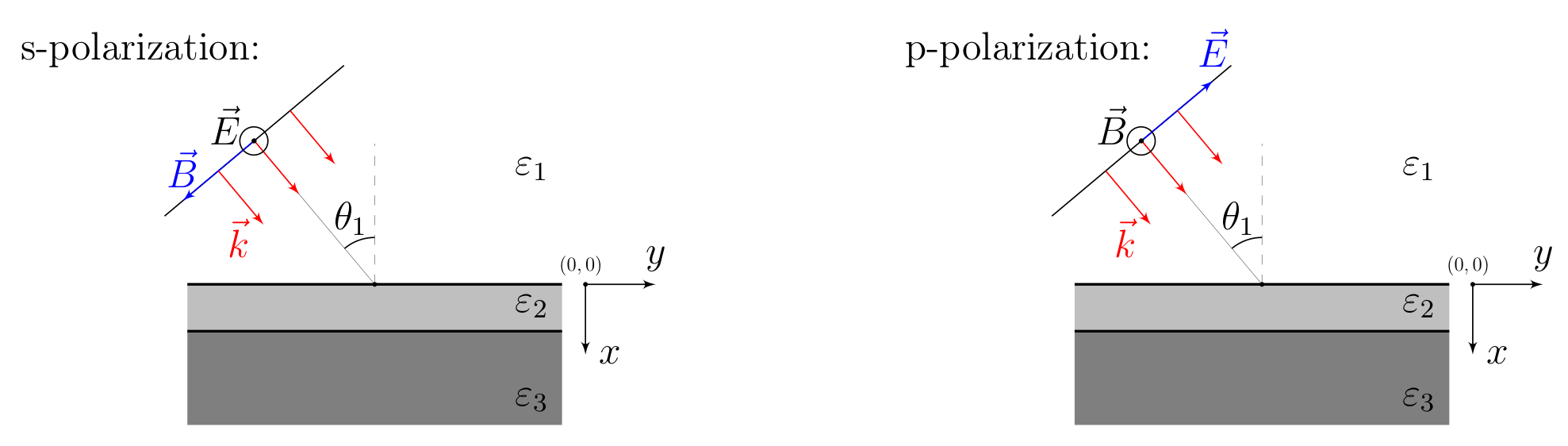
When a incident wave falls on the film, a reflected wave occurs in the medium $\varepsilon_1$ , a passing wave in the medium $\varepsilon_3$ and a superposition of waves going in different directions in the medium $\varepsilon_2$ . In $s$ -polarization, the direction of the electric field is fixed, so we can proceed to consider scalar complex amplitudes:

\begin{cases} \tilde{E}_1 = \mathcal{E}e^{ik_{1x}x + ik_{1y}y} + r \cdot \mathcal{E}e^{-ik_{1x}x + ik_{1y}y} \\ \tilde{E}_2 = a \cdot \mathcal{E}e^{ik_{2x}x + ik_{2y}y} + b \cdot \mathcal{E}e^{-ik_{2x}x + ik_{2y}y} \\ \tilde{E}_3 = t \cdot \mathcal{E}e^{ik_{3x}(x-d) + ik_{3y}y} \end{cases}

In $p$ -polarization, the direction of the magnetic field is fixed, so it is easier to proceed to the consideration of scalar complex amplitudes of the magnetic field:

\begin{cases} \tilde{B}_1 = \mathcal{B}e^{ik_{1x}x + ik_{1y}y} + r \cdot \mathcal{B}e^{-ik_{1x}x + ik_{1y}y} \\ \tilde{B}_2 = a \cdot \mathcal{B}e^{ik_{2x}x + ik_{2y}y} + b \cdot \mathcal{B}e^{-ik_{2x}x + ik_{2y}y} \\ \tilde{B}_3 = t \cdot \mathcal{B}e^{ik_{3x}(x-d) + ik_{3y}y} \end{cases}

Two side-by-side diagrams (s-polarization: and p-polarization:) of a wave incident at angle θ1 from medium ε1 onto a film ε2 over a substrate ε3; wave vector k in red, the field perpendicular to the plane drawn as a circled dot (E for s, B for p) and the other field in blue (B for s, E for p); axes y to the right and x downward from the origin (0,0). — The incidence of the $s$ -polarized and $p$ -polarized wave on the film

A1 Show that $k_{1y} = k_{2y} = k_{3y}$ .

A2 Find expressions for $k_{1x}$ , $k_{2x}$ and $k_{3x}$ in terms of $\omega$ , $c$ , $\theta_1$ , $\varepsilon_1$ , $\varepsilon_2$ , $\varepsilon_3$ .

A3 For a wave with $s$ -polarization (the electric field is directed along the surface), from the boundary conditions for the tangential components of the fields, obtain a system of linear equations for the coefficients $r$ , $A$ , $b$ and $t$ .

A4 Find the reflection coefficient. Bring the answer to the form:

r_s = \frac{A + Be^{2ik_{2x}d}}{AB + e^{2ik_{2x}d}}.

Express the real numbers $A$ , $B$ in terms of $k_{1x}$ , $k_{2x}$ and $k_{3x}$ .

For convenience, use the variables $\kappa_{ix} = \dfrac{k_{ix}}{\varepsilon_i}$ for $i \in [1, 3]$ .

A5 For a wave with $p$ -polarization (the magnetic field is directed along the surface), from the boundary conditions for the tangential components of the fields, obtain a system of linear equations for the coefficients $r$ , $A$ , $b$ and $t$ .

A6 Find the reflection coefficient. Bring the answer to the form:

r_p = \frac{A + Be^{2ik_{2x}d}}{AB + e^{2ik_{2x}d}}.

Express the real numbers $A$ , $B$ in terms of $k_{1x}$ , $k_{2x}$ and $k_{3x}$ .

We will perform preliminary calculations of the approximate shape of the ellipsometric spectrum of a thin layer of silicon dioxide on a silicon substrate. Until the end of Part A, we will neglect the optical dispersion, and assume $\varepsilon_{\mathrm{Air}} = 1.00$ , $\varepsilon_{\mathrm{Si}} = 17.2 - 0.430i$ , $\varepsilon_{\mathrm{SiO_2}} = 2.13$ . Note that silicon has an imaginary part of the dielectric constant responsible for absorption, due to which it is opaque. The use of complex permittivity does not change obtained expressions, if the trigonometric functions of the complex parameter are considered.

With the help of the A.py program, you can plot $\Psi$ and $\Delta$ for different angles of incidence $\theta_1$ and thicknesses $d$ . At the input, the program receives the name Name of the series, the angle of incidence $\theta_1$ from the air (in degrees) and the thickness $d$ of the dioxide film in the form of a table written in the file A_in.txt .

There is an example of filling in a table in a file A_in.txt:

Name	$\theta_1,^{\circ}$	$d,\ \mathrm{nm}$
ex1	50	40
ex2	30	100
⋮	⋮	⋮

The input data is limited to $20^{\circ} \le \theta_1 \le 80^{\circ}$ , $d \le 250$ nm. The name of the experiment should not contain spaces and tabs. The separator between the integer and fractional parts of numbers is a dot. The separator between the columns is a tab.

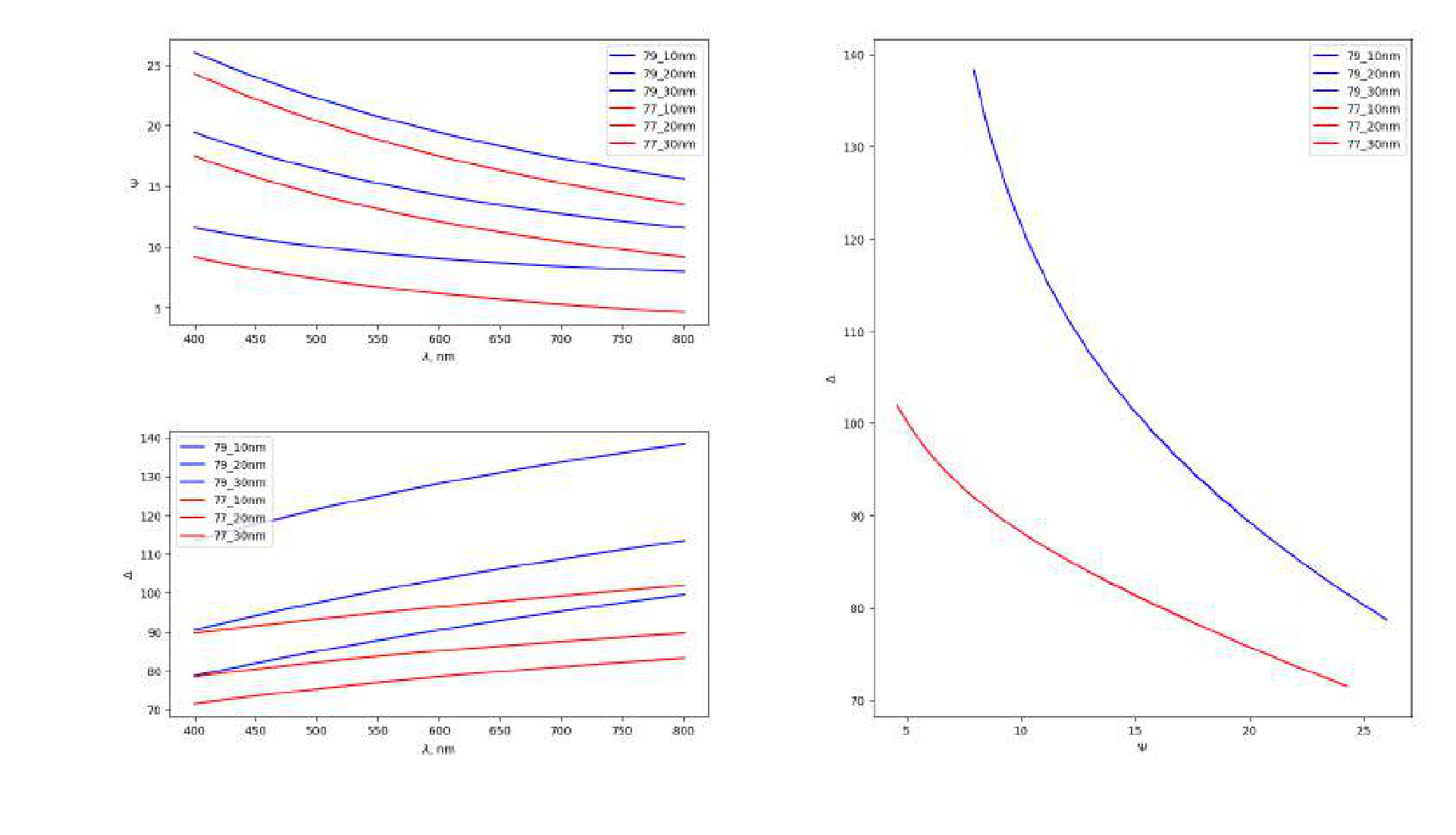
A7 Using the program A.py plot the dependence of $\Psi$ and $\Delta$ on $\lambda$ at different angles of incidence $\theta_1$ and thicknesses $d$ . Conduct a quantitative study and determine at which angle of incidence $\theta_{\mathrm{opt}}$ the ellipsometric angle $\Psi$ is most sensitive (the highest value $|\Delta\Psi/\Delta d|$ ) to changes in $d$ in the range from $10\,\mathrm{nm}$ to $50\,\mathrm{nm}$ . Find the value of $\theta_{\mathrm{opt}}$ with an accuracy of one degree.
Since B3, use $\theta_{opt}$ as $\Phi$ to increase accuracy.

Part B. Kinetics of oxidation

In this part, the angle of incidence of the beam on the film will be indicated by $\Phi$ .

Together with a colleague, you are studying the deposition of thin oxide films on the surface of silicon during prolonged calcination in the dry air. Real silicon Si and silicon dioxide $\mathrm{SiO_2}$ have optical dispersion, so the graphs $\Psi, \Delta$ from $\lambda$ that will be offered to you in this part may slightly differ from those that you built in the part A7.

Attention! The optical dispersion of Si and $\mathrm{SiO_2}$ is automatically embedded in all programs that you will work with in this part.

Your colleague was working late on the ellipsometer yesterday and forgot to write down the value of the angle $\Phi$ . He measured the thickness of the oxide film on two samples and transmitted the measurement results to you in files B1.txt and B2.txt.

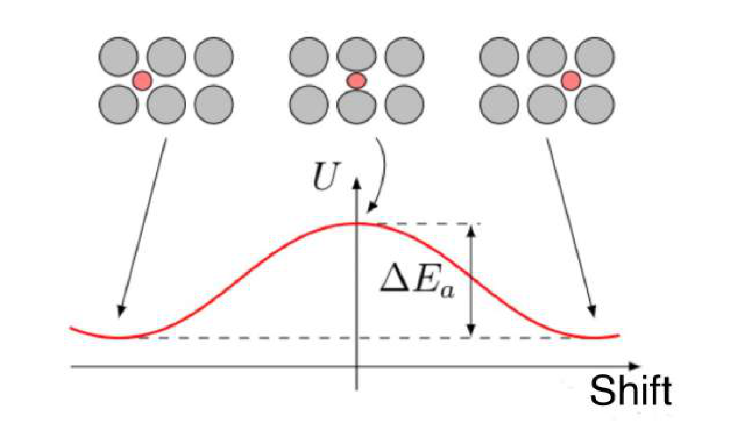
Three snapshots of a small red atom moving between grey lattice atoms (left position, squeezed between two atoms in the middle, right position), with arrows to a red potential-energy curve U versus Shift: minima at the sides and a maximum in the middle; the barrier height is marked ΔEa. — A qualitative diffusion scheme in a solid and the meaning of energy $\Delta E_a$ .

B1 Using the program B1.py find by hand the value $\Phi$ and the thickness $d$ of $\mathrm{SiO_2}$ film. The program B1.py reads values from a file B1.txt automatically and outputs an approximating graph $\Psi, \Delta$ from $\lambda$ , for the values of the angle $\Phi$ entered by you in degrees and the thickness $d$ of the dioxide film in nanometers. The input data is limited: $20^{\circ} \le \Phi \le 80^{\circ}$ , $d \le 250$ nm.

B2 Using the program B2.py find by hand the value $\Phi$ and the thickness $d$ of $\mathrm{SiO_2}$ film. The program works similarly to the previous B1.

For a detailed study of the oxidation rate, you can get ellipsometric data from your colleague, measured from a real-time oxidizing silicon substrate. At the initial moment $t = 0$ , he puts pure silicon inside the furniture with a temperature $T$ , and every 2 min mesures the spectrum $\Psi, \Delta$ from $\lambda$ at a fixed angle $\Phi$ , which you tell him.

In the file B_in.txt you specify the name of the experiment, the angle $\Phi$ in degrees, the temperature $T$ in degrees Celsius, and the duration of the experiment in minutes in the form of a table:

Name	$\Phi,^{\circ}$	$T,^{\circ}\mathrm{C}$	$t,\ \mathrm{min}$
test	50	1000	40
⋮	⋮	⋮	⋮

The input data is limited as $20^{\circ} \le \Phi \le 80^{\circ}$ , $800\,{}^{\circ}\mathrm{C} \le T \le 1200\,{}^{\circ}\mathrm{C}$ , $t \le 200$ min. The name of the experiment should not contain spaces and tabs. The separator between the integer and fractional parts of a number is a dot. The separator between the columns is a tab. Next, you run the program gen_data.exe which simulates your colleague conducting an experiment in accelerated mode. You can interrupt the execution of this program at any time, and the results of the measurements already performed will be saved on your computer. You can automatically process the measurement data using the program B.py which uses the same file B_in.txt . This program uses the results of the work gen_data.exe, selects the value of $d$ for each point and calculates the statistical error of this value. Keep in mind that processing may take several minutes. The results of the program B.py are located in the /res folder in the form of tables and graphs $d(t)$ . An example of an automatically generated program B.py tables in the /res folder:

$t,\ \mathrm{min}$	$d,\ \mathrm{nm}$	$\Delta d,\ \mathrm{nm}$
2	17.3	0.3
⋮	⋮	⋮

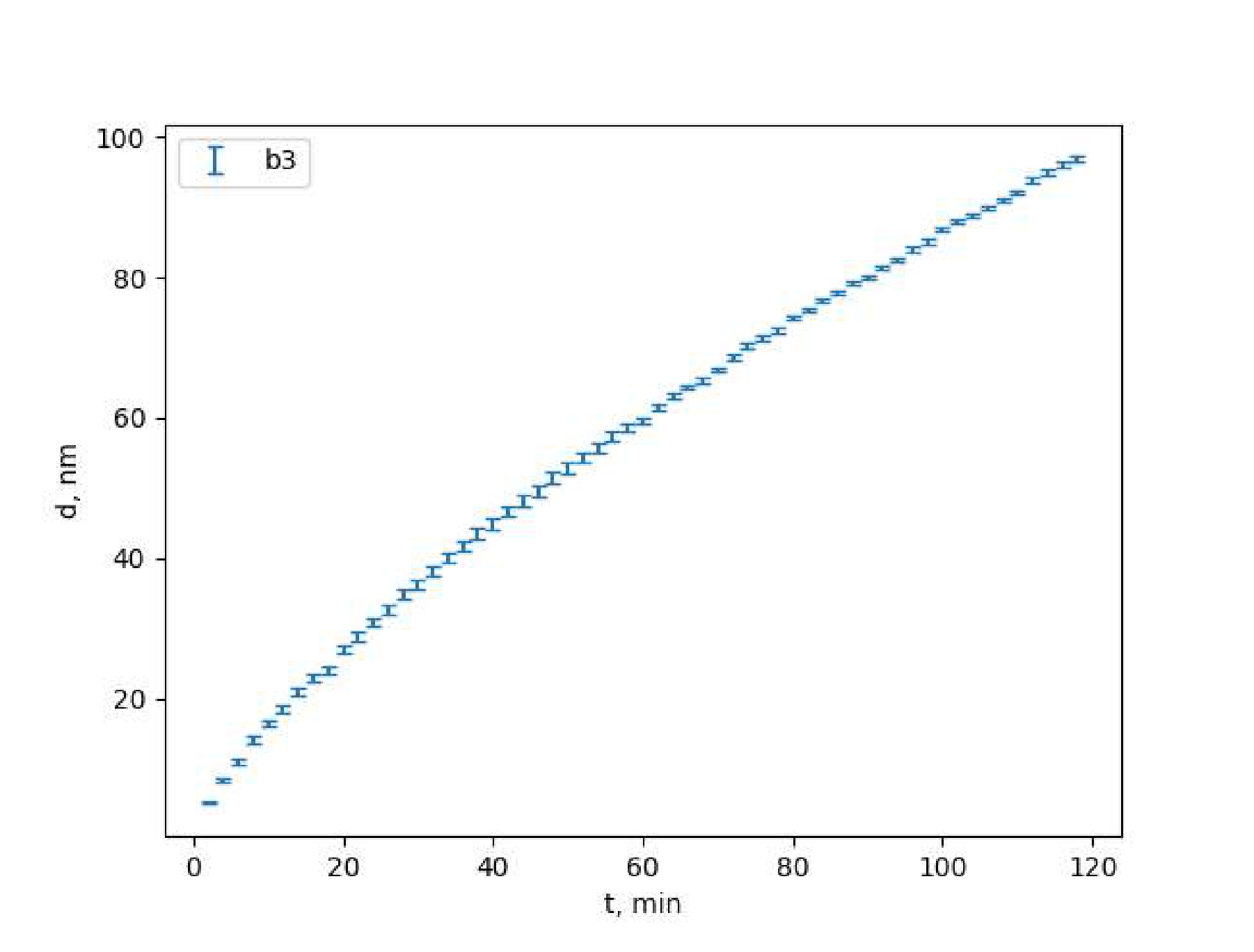
B3 Get the data for the dependence of the film thickness $d$ of silicon dioxide on the time $t$ during oxidation at a temperature of $t = 1000\,{}^{\circ}\mathrm{C}$ for 120 min. Attach the graph obtained by the program B.py to the report.

Now let us consider the theoretical aspects of thermal oxidation. According to the Deal-Grove model, three processes are responsible for the rate of increase in the thickness of the silicon oxide layer:

diffusion of oxygen to the surface $\mathrm{SiO_2}$ ;
diffusion of oxygen through the layer $\mathrm{SiO_2}$ ;
oxidation reaction $\mathrm{Si} + \mathrm{O_2} \to \mathrm{SiO_2}$ at the interface $\mathrm{SiO_2/Si}$ .

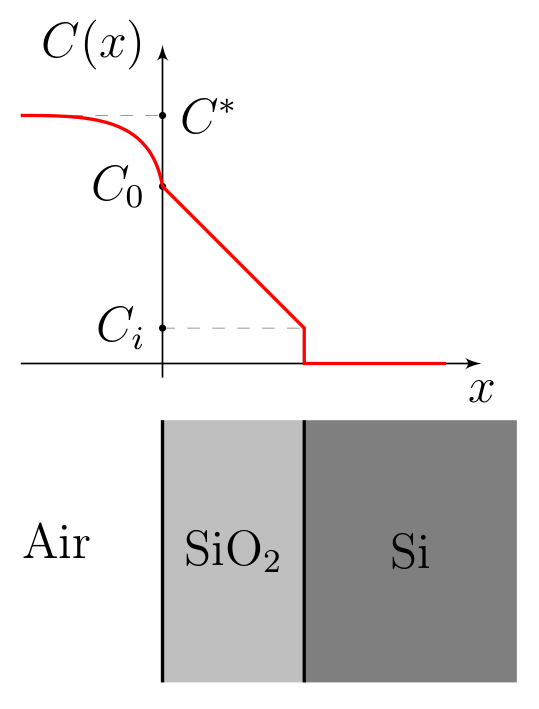
Thus, the concentration of oxygen $C$ (dimension $\mathrm{mol/m^3}$ ) changes as it moves deeper into the sample. In the air, far away from the substrate, the oxygen concentration is $C^*$ ; inside the silicon dioxide layer, the concentration decreases linearly from $C_0$ to $C_i$ ; inside silicon, the oxygen concentration is zero.

Let us consider a model for describing these processes. Specific (i.e. per unit surface area) the flow rates of each of the three processes $F_1$ , $F_2$ , $F_3$ (units of measurement — $\mathrm{mole/(c \cdot m^2)}$ ) we define as follows:

The diffusion rate is $F_1 = h(C^* - C_0)$ , where $h$ is a certain coefficient characterizing diffusion in the gas phase.
Counting the diffusion rate $F_2 = \frac{D}{d}(C_0 - C_i)$ , where $D$ is the diffusion coefficient of oxygen in the dioxide, depending on the temperature $T$ , and $d$ is the thickness of the silicon dioxide film.
The rate of the oxidation reaction $F_3 = kC_i$ , where $k$ is the constant of the rate of the oxidation reaction, depending on the temperature $T$ .

B4 Express the growing velocity $v$ of film thickness change in terms of the oxidation reaction rate $F_3$ , the molar mass $\mu_{\mathrm{SiO_2}}$ and the density $\rho_{\mathrm{SiO_2}}$ of silicon dioxide. Assume that the air-dioxide boundary does not move.

B5 Assuming the problem to be quasi-stationary (the establishment times of all processes are much less than the film rise time), express $C_0$ and $C_i$ in terms of $C^*$ , the velocity constants $h$ , $k$ , $D$ and the film thickness $d$ .

B6 Get the differential equation for the thickness $d$ of the dioxide film and get its solution with the initial condition $d(t_0) = d_0$ in the form

d^2 + Ad = B(t + \tau),

where $\tau$ contains information about the initial conditions, and the constants $A$ and $B$ are related to the kinetics of oxidation. Express $A$ and $B$ in terms of $h$ , $k$ , $D$ , $C^*$ , $\mu_{\mathrm{SiO_2}}$ and $\rho_{\mathrm{SiO_2}}$ .

Experiments show that blowing with air (changing the profile $C(x)$ above the surface), doesn’t change the rate of the process. Therefore we will consider $h \gg k$ .

At the beginning of the oxidation process, the stationary model is not applicable, so it is used starting from the minimum thickness $d_0 = 25$ nm. Enter into the program B7.py the data from the file B_in.txt and get the parameters $B$ and $B/A$ automatically. If the maximum film thickness obtained in the experiment is less than $d_0$ , then the program B7.py outputs ”Final layer is too thin to approximate”.

If the program returns the error ”FileNotFoundError”, run the files gen_data.exe and B.py sequentially with the input data you need, previously entered in the B_in.txt.

B7 Get the values of the parameters $B$ and $B/A$ for five different temperatures $T$ . Save the results into a file B8_in.txt in the form of a table.

$T,^{\circ}\mathrm{C}$	$B,\ \mathrm{nm^2/min}$	$\Delta B,\ \mathrm{nm^2/min}$	$B/A,\ \mathrm{nm/min}$	$\Delta(B/A),\ \mathrm{nm/min}$
1000	174	4	1.21	0.02
⋮	⋮	⋮	⋮	⋮

The dependence of the reaction rate constant $k$ on temperature $T$ is associated with the energy $\Delta E_b$ of breaking the bond $\mathrm{Si - Si}$ in a silicon crystal, and then the relation between them:

k \propto e^{-\Delta E_b/k_B T}.

The diffusion coefficient in solids is also related to temperature via the so-called activation energy $\Delta E_a$ , and the quantitative dependence has the form:

D \propto e^{-\Delta E_a/k_B T}

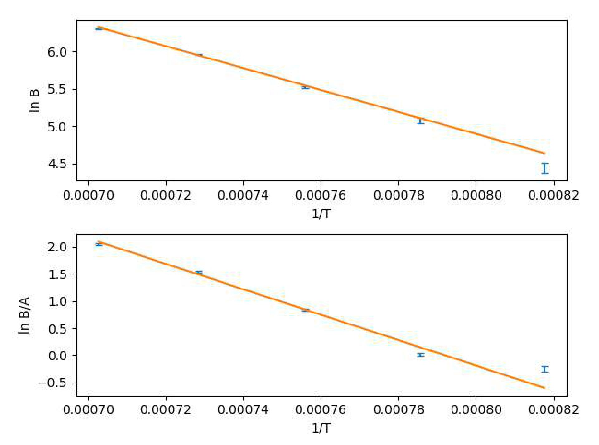
Using the program B8.py you can plot graphs $\ln(B \cdot \mathrm{min/nm^2})$ from $1/T$ and $\ln(B/A \cdot \mathrm{min/nm})$ from $1/T$ and determine the parameters of the automatically drawn lines.

Boltzmann constant $k_B = 1.38 \cdot 10^{-23}$ J/C, elementary charge $e = 1.60 \cdot 10^{-19}$ C.

B8 Determine the values of $\Delta E_b$ and $\Delta E_a$ in electron volts. Attach the linearized graphs to the report.

Отговори

Решение

Part A. Theoretical principles of ellipsometry

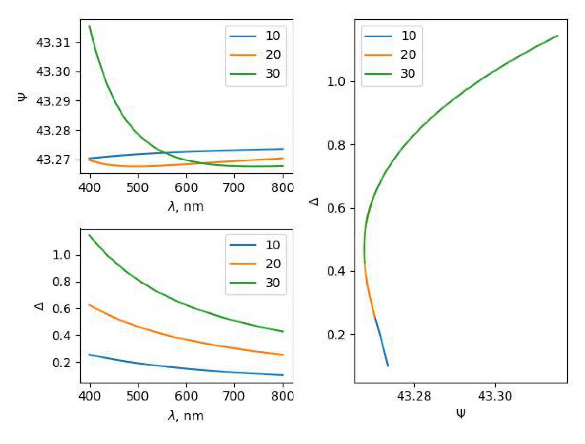
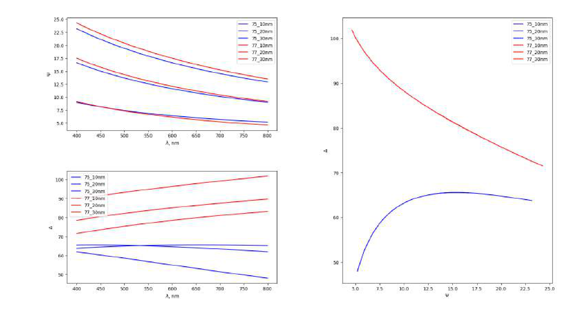
Three plots for thicknesses 10, 20, 30 (legend): Ψ versus λ, nm (about 43.27–43.31), Δ versus λ, nm (about 0.1–1.15), and Δ versus Ψ (right, tall panel). — Dependencies for the angle of incidence of $20^{\circ}$ and film thicknesses of 10 nm, 20 nm and 30 nm.

Three plots with blue curves 75_10nm, 75_20nm, 75_30nm and red curves 77_10nm, 77_20nm, 77_30nm: Ψ versus λ, nm; Δ versus λ, nm; and Δ versus Ψ. — A comparison of the dependencies for the angles of incidence of $75^{\circ}$ and $77^{\circ}$ and the film thickness of 10 nm, 20 nm and 30 nm.

Three plots with blue curves 79_10nm, 79_20nm, 79_30nm and red curves 77_10nm, 77_20nm, 77_30nm: Ψ versus λ, nm; Δ versus λ, nm; and Δ versus Ψ. — A comparison of the dependencies for the angles of incidence of $77^{\circ}$ and $79^{\circ}$ and the film thickness of 10 nm, 20 nm and 30 nm.

A1 A given system of equations for scalar complex amplitudes must be performed at any point of the interface between media:

\forall y \quad E_y(x=-0) = E_y(x=+0); \begin{cases} E_y(x=-0) = f \cdot e^{-ik_{1y}y},\ f \ne f(y), \\ E_y(x=+0) = g \cdot e^{-ik_{2y}y},\ g \ne g(y). \end{cases}

This necessarily follows $k_{1y} = k_{2y}$ . Similarly, considering the second boundary, we obtain $k_{2y} = k_{3y}$ .

A2 Using the expression for $k$ and the equality $k_y = k_{1y} = k_{2y} = k_{3y}$ :

k = \sqrt{k_{1x}^2 + k_y^2} \Rightarrow k_{1x} = \sqrt{\frac{\varepsilon_1\omega^2}{c^2} - k_y^2} = \frac{\sqrt{\varepsilon_1}\omega}{c}\cos\theta_1.

Similarly,

k_{2x} = \frac{\sqrt{\varepsilon_2}\omega}{c}\cos\theta_2 = \frac{\sqrt{\varepsilon_2}\omega}{c}\sqrt{1 - \frac{\varepsilon_1}{\varepsilon_2}\sin^2\theta_1},

k_{3x} = \frac{\sqrt{\varepsilon_3}\omega}{c}\cos\theta_3 = \frac{\sqrt{\varepsilon_3}\omega}{c}\sqrt{1 - \frac{\varepsilon_1}{\varepsilon_3}\sin^2\theta_1}.

\boxed{\begin{cases} k_{1x} = \dfrac{\sqrt{\varepsilon_1}\omega}{c}\cos\theta_1, \\ k_{2x} = \dfrac{\omega}{c}\sqrt{\varepsilon_2 - \varepsilon_1\sin^2\theta_1}, \\ k_{3x} = \dfrac{\omega}{c}\sqrt{\varepsilon_3 - \varepsilon_1\sin^2\theta_1} \end{cases}}

A3 Let’s write down the boundary conditions for boundary 1-2 on the tangential components $E$ and $B$ , respectively, counting $x = 0$ :

\mathcal{E} + r\mathcal{E} = a\mathcal{E} + b\mathcal{E},

k_{1x}\mathcal{E} - k_{1x}\mathcal{E}r = k_{2x}a\mathcal{E} - k_{2x}b\mathcal{E}.

And for the boundary 2-3:

a\mathcal{E}e^{ik_{2x}d} + b\mathcal{E}e^{-ik_{2x}d} = t\mathcal{E}\ ,

k_{3x}t\mathcal{E} = k_{2x}\mathcal{E}ae^{ik_{2x}d} - k_{2x}\mathcal{E}be^{-ik_{2x}d}.

Thus, we obtained a system of equations:

\begin{cases} 1 + r = a + b, \\ k_{1x}(1 - r) = k_{2x}(a - b), \\ ae^{i\phi} + be^{-i\phi} = t, \\ k_{3x}t = k_{2x}(ae^{i\phi} - be^{-i\phi}), \end{cases}

where the notation $\phi = k_{2x}d$ is introduced.

\boxed{\begin{cases} 1 + r = a + b, \\ k_{1x}(1 - r) = k_{2x}(a - b), \\ ae^{ik_{2x}d} + be^{-ik_{2x}d} = t, \\ k_{3x}t = k_{2x}(ae^{ik_{2x}d} - be^{-ik_{2x}d}). \end{cases}}

A4 From the A3, we get:

\begin{cases} t = (ae^{i\psi} - be^{-i\psi})\dfrac{k_{2x}}{k_{3x}}, \\ a = be^{-2i\psi} \cdot \dfrac{k_{2x} + k_{3x}}{k_{2x} - k_{3x}}, \\ a(k_{1x} + k_{2x}) + b(k_{1x} - k_{2x}) = 2k_{1x}, \\ r = \dfrac{a(k_{1x} - k_{2x}) + b(k_{1x} + k_{2x})}{2k_{1x}}. \end{cases}

Deciding, we come to the result:

r_s = \frac{(k_{1x} - k_{2x})(k_{2x} + k_{3x}) + (k_{1x} + k_{2x})(k_{2x} - k_{3x})e^{2i\phi}}{(k_{1x} - k_{2x})(k_{2x} - k_{3x})e^{2i\phi} + (k_{1x} + k_{2x})(k_{2x} + k_{3x})}.

Introducing the notation

\boxed{\begin{cases} A = \dfrac{k_{2x} + k_{3x}}{k_{2x} - k_{3x}}, \\ B = \dfrac{k_{1x} + k_{2x}}{k_{1x} - k_{2x}}. \end{cases}}

we get the expression reduced to the required form.

A5 Similarly, A3 records the conditions at the two interfaces, taking into account the connection of electric and magnetic fields in the EM wave: $\sqrt{\varepsilon\varepsilon_0\mu_0}\mathcal{E} = \mathcal{B}$ :

\begin{cases} 1 + r = a + b, \\ \dfrac{k_{1x}}{\varepsilon_1}(1 - r) = \dfrac{k_{2x}}{\varepsilon_2}(a - b), \\ ae^{ik_{2x}d} + be^{-ik_{2x}d} = t, \\ \dfrac{k_{3x}}{\varepsilon_3}t = \dfrac{k_{2x}}{\varepsilon_2}(ae^{ik_{2x}d} - be^{-ik_{2x}d}). \end{cases}

Or, taking into account the reinterpretations proposed in the condition:

\boxed{\begin{cases} 1 + r = a + b, \\ \kappa_{1x}(1 - r) = \kappa_{2x}(a - b), \\ ae^{i\phi} + be^{-i\phi} = t, \\ \kappa_{3x}t = \kappa_{2x}(ae^{i\phi} - be^{-i\phi}) \end{cases}}

A6 Note that the system in A5 coincides with the system from A3 up to the replacement of $\kappa_{ix} \leftrightarrow k_{ix}$ . Accordingly, we immediately write down the answer:

r_p = \frac{A + Be^{2i\phi}}{AB + e^{2\phi}},

\boxed{\begin{cases} A = \dfrac{\kappa_{2x} + \kappa_{3x}}{\kappa_{2x} - \kappa_{3x}}, \\ B = \dfrac{\kappa_{1x} + \kappa_{2x}}{\kappa_{1x} - \kappa_{2x}}. \end{cases}}

A7 We will receive graphs for three thicknesses: 10, 20 and 30 nm. At low angles of incidence, it can be seen that the maximum range of $\Psi$ is hundredths degrees, while $\theta \sim 70^{\circ}$ , the maximum range of $\Phi$ is tens of degrees . The maximum sufficiency is reached when

\theta_{\mathrm{opt}} = 77^{\circ}.

The corresponding graphs for comparison are given below.

\boxed{\theta_{\mathrm{opt}} = 77^{\circ}}

Part B. Kinetics of oxidation

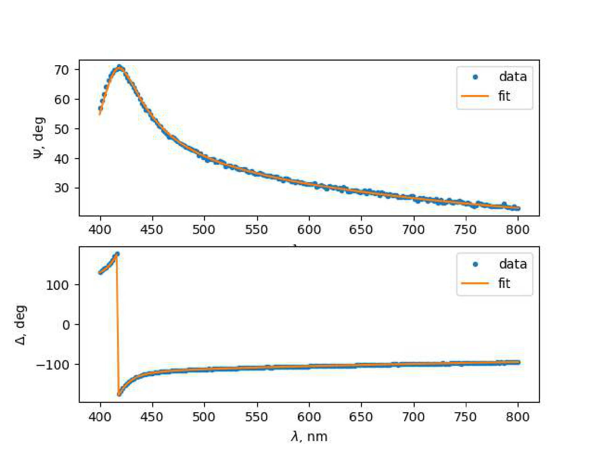
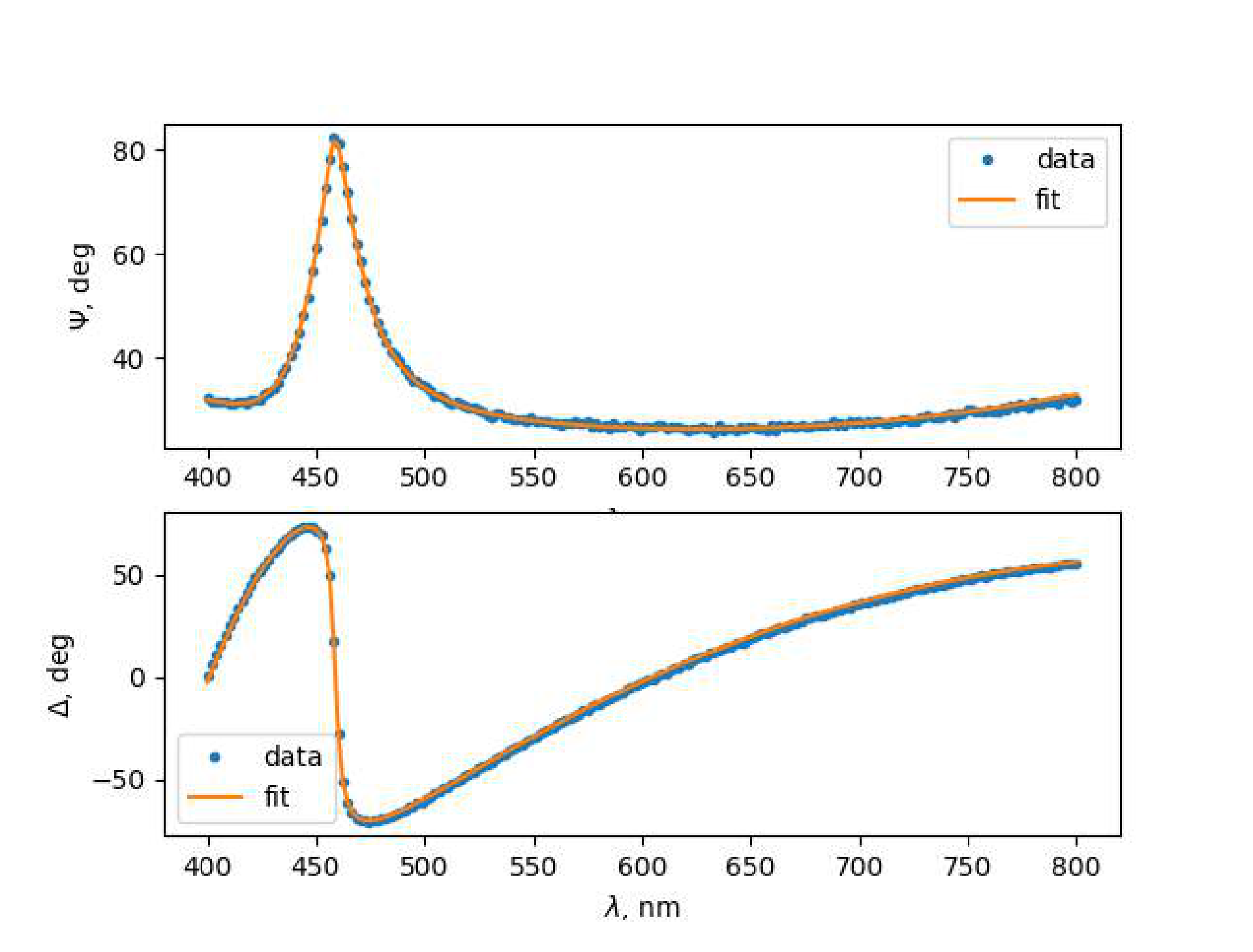
Two stacked plots versus λ, nm from 400 to 800 with data points and fit (legend data/fit): Ψ, deg with a peak of about 70 near 420 nm then decreasing to about 23; Δ, deg rising to about 175 near 418 nm, jumping to about −170 and then slowly rising to about −95. — The graph for $\Phi = 71^{\circ}, d = 67\,\mathrm{nm}$ .

Two stacked plots versus λ, nm from 400 to 800 with data points and fit (legend data/fit): Ψ, deg with a sharp peak of about 82 near 458 nm; Δ, deg rising to about 73 near 450 nm, falling to about −70 near 475 nm and then rising to about 55 at 800 nm. — The graph for $\Phi = 57^{\circ}, d = 232\,\mathrm{nm}$ .

Plot of d, nm versus t, min (0 to 120) for series b3: points with small error bars rising from about 5 nm at 2 min to about 97 nm at 118 min along a concave curve.

Two plots versus 1/T from 0.00070 to 0.00082 with error-bar points and an orange fitted line: ln B decreasing from about 6.3 to about 4.4, and ln B/A decreasing from about 2.05 to about −0.25.

B1 Let us describe the search algorithm for optimal $\Phi$ and $d$ . First enter arbitrary $\Phi$ and $d$ in B1.py. Next, on each step we try to change $\Phi$ or $d$ a bit, and look at the "error" given out by the program B1.py. If the error decreases, we continue to change $\Phi$ or $d$ in the same direction (e.g. if we have lowered $\Phi$ by $1^{\circ}$ , and the error have decreased, then on the next step we also lower $\Phi$ by $1^{\circ}$ ). Finally, we will reach such $\Phi$ and $d$ that any small changes of them lead to the increasing of the error, i.e. we reach the minimal possible error. It means that we have found optimal $\Phi$ and $d$ .

One can see on the graph how fitting data correspond to the colleague’s ones, but the numerical parameter of the approximation quality is the error giving by the program B1.py.

\boxed{\Phi = 71.1^{\circ} \quad d = 66.7\ \mathrm{nm}}

B2 The search algorithm for optimal $\Phi$ and $d$ coincides with the such one in part B1.

\boxed{\Phi = 57^{\circ} \quad d = 232\ \mathrm{nm}}

B3 Set name = b3, Phi = 77, $T = 1000$ , $t_{\max} = 120$ in B_in.txt, then run gen_data.exe and B.py consistently. In "res" folder we get the file with desired graph. Note that we substitute $\Phi = \theta_{\mathrm{opt}}$ from A7 in order to increase the quality of the experiment.

B4 Consider a small time period $\Delta t$ and a part of $\mathrm{SiO_2}$ -Si border having the area $S$ . Then the mass of the Si oxided during $\Delta t$ equals $\Delta m = F_3\,\Delta t\,S\,\mu_{\mathrm{SiO_2}}$ . On the other hand, the $\mathrm{SiO_2}$ -Si border will move by $v\,\Delta t$ , so the mass of $\mathrm{SiO_2}$ appeared equals $\Delta m = \rho_{\mathrm{SiO_2}}\,S\,v\,\Delta t$ . Thus $\rho_{\mathrm{SiO_2}}\,v\,S\,\Delta t = F_3\,\Delta t\,S\,\mu_{\mathrm{SiO_2}}$ , so $\rho_{\mathrm{SiO_2}}\,v = F_3\,\mu_{\mathrm{SiO_2}}$ .

\boxed{v = F_3\frac{\mu_{\mathrm{SiO_2}}}{\rho_{\mathrm{SiO_2}}}}

B5 Stationarity conditions gives $F_1 = F_2 = F_3$ , i.e. $h(C^* - C_0) = \frac{D}{d}(C_0 - C_i) = kC_i$ . From the second equality we get $C_0 = (1 + \frac{kd}{D})C_i$ . Substitute it in $h(C^* - C_0) = kC_i$ and get $h(C^* - (1 + \frac{kd}{D})C_i) = kC_i$ , what implies $C^* = (\frac{k}{h} + \frac{kd}{D} + 1)C_i$ , so

C_i = \frac{C^*}{1 + \frac{k}{h} + \frac{kd}{D}}, \quad C_0 = \left(1 + \frac{kd}{D}\right)C_i = C^*\frac{1 + \frac{kd}{D}}{1 + \frac{k}{h} + \frac{kd}{D}}

\boxed{C_0 = C^*\frac{1 + \dfrac{kd}{D}}{1 + \dfrac{k}{h} + \dfrac{kd}{D}}, \qquad C_i = C^*\frac{1}{1 + \dfrac{k}{h} + \dfrac{kd}{D}}}

B6 From B4 we have $v = \dot{d} = \frac{F_3\mu_{\mathrm{SiO_2}}}{\rho_{\mathrm{SiO_2}}} = \frac{kC_i\mu_{\mathrm{SiO_2}}}{\rho_{\mathrm{SiO_2}}}$ . Taking into account the expression for $C_i$ obtained in B5 we get

\dot{d} = C^*\frac{\mu_{\mathrm{SiO_2}}}{\rho_{\mathrm{SiO_2}}}\frac{1}{\frac{1}{k} + \frac{1}{h} + \frac{d}{D}}

or, equivalently,

\frac{\dot{d} \cdot d}{D} + \dot{d} \cdot \left(\frac{1}{k} + \frac{1}{h}\right) - C^*\frac{\mu_{\mathrm{SiO_2}}}{\rho_{\mathrm{SiO_2}}} = 0

Note that the left hand side equals

\frac{d}{dt}\left(\frac{d^2}{2D} + d \cdot \left(\frac{1}{k} + \frac{1}{h}\right) - t \cdot C^*\frac{\mu_{\mathrm{SiO_2}}}{\rho_{\mathrm{SiO_2}}}\right) = 0

\frac{d^2}{2D} + d \cdot \left(\frac{1}{k} + \frac{1}{h}\right) - t \cdot C^*\frac{\mu_{\mathrm{SiO_2}}}{\rho_{\mathrm{SiO_2}}} = \mathrm{const}

where const can be found from the initial condition $d(t_0) = d_0$ . Namely,

\mathrm{const} = \frac{d_0^2}{2D} + d_0 \cdot \left(\frac{1}{k} + \frac{1}{h}\right) - t_0 \cdot C^*\frac{\mu_{\mathrm{SiO_2}}}{\rho_{\mathrm{SiO_2}}}

So we get

d^2 + 2D \cdot \left(\frac{1}{k} + \frac{1}{h}\right) \cdot d = 2DC^*\frac{\mu_{\mathrm{SiO_2}}}{\rho_{\mathrm{SiO_2}}}(t + \tau)

where $\tau = \frac{\mathrm{const} \cdot \rho_{\mathrm{SiO_2}}}{2DC^*\mu_{\mathrm{SiO_2}}}$ .

\boxed{A = 2D\left(\frac{1}{k} + \frac{1}{h}\right), \quad B = 2DC^*\frac{\mu_{\mathrm{SiO_2}}}{\rho_{\mathrm{SiO_2}}}}

B7 First create data necessary for B7.py. Set $T$ , $\Phi = \theta_{\mathrm{opt}} = 77^{\circ}$ , $t_{\max} = 120$ in B_in.txt, then run gen_data.exe and B.py, and finally, run B7.py five times, on each time entering name, $T$ and $\Phi$ from B_in.txt. We write every output of B7.py in the file B8_in.txt and get the table below.

Note that even for $T = 850^{\circ}C$ we get an error "Final layer is too thin to approximate", and for $T = 900^{\circ}C$ we get too high error rate, so it is reasonable to start with $T = 950^{\circ}C$ with a step $50^{\circ}C$ .

$T,\ {}^{\circ}C$	$B,\ \mathrm{nm^2/min}$	$\Delta B,\ \mathrm{nm^2/min}$	$B/A,\ \mathrm{nm/min}$	$\Delta(B/A),\ \mathrm{nm/min}$
950	85	6	0.780	0.044
1000	160	6	1.017	0.027
1050	251	4	2.310	0.044
1100	389	2	4.636	0.070
1150	551	4	7.751	0.188

B8 First plot the graphs $\ln B\left(\frac{1}{T}\right)$ and $\ln\frac{B}{A}\left(\frac{1}{T}\right)$ using the program B8.py. In the console one can see the slopes of proposed linear approximations. Namely, the slope coefficient of $\ln B\left(\frac{1}{T}\right)$ equals $-(14671 \pm 625)\,{}^{\circ}C$ , and the slope coefficient of $\ln\frac{B}{A}\left(\frac{1}{T}\right)$ equals $-(23418 \pm 1730)\,{}^{\circ}C$ (where $K$ means one kelvin).

We get from B6 that

B = 2DC^*\frac{\mu_{\mathrm{SiO_2}}}{\rho_{\mathrm{SiO_2}}} \propto e^{-\frac{\Delta E_a}{k_B T}}

Thus the slope coefficient of the graph $\ln B\left(\frac{1}{T}\right)$ equals $-\frac{\Delta E_a}{k_B}$ . So $\Delta E_a = (2.208 \pm 0.086) \cdot 10^{-19}$ J, or, equivalently,

\Delta E_a = \frac{(2.208 \pm 0.086) \cdot 10^{-19}}{1.60 \cdot 10^{-19}}\,eV = (1.38 \pm 0.05)\,eV

Next, $h \gg k$ implies $A \approx \frac{2D}{k}$ , so

\frac{B}{A} \approx kC^*\frac{\mu_{\mathrm{SiO_2}}}{\rho_{\mathrm{SiO_2}}} \propto e^{-\frac{\Delta E_b}{k_B T}}

the slope coefficient of the graph $\ln\frac{B}{A}\left(\frac{1}{T}\right)$ equals $-\frac{\Delta E_b}{k_B}$ . So $\Delta E_b = (3.23 \pm 0.23) \cdot 10^{-19}$ J, or, equivalently,

\Delta E_b = \frac{(3.23 \pm 0.23) \cdot 10^{-19}}{1.60 \cdot 10^{-19}}\,eV = (2.02 \pm 0.14)\,eV

\boxed{\Delta E_a = (1.38 \pm 0.05)\,eV, \quad \Delta E_b = (2.02 \pm 0.14)\,eV}

Оригинал в Архива: T1.pdf · официални решения: T1_sol.pdf