Съдържание
УсловиеInstructions for using the FBG-Writer softwarePart A. FBG fabrication technology (5 т.)Part B. Coupled mode theory (2,9 т.)Part C. Calibration of an FBG temperature sensor (2,9 т.)Part D. Using the FBG temperature sensor (2,4 т.)Part E. FBG dynamometer (3,9 т.)Part F. Birefringence in FBG (2,9 т.)РешениеISPhO 2026, Експеримент — Задача 1. Fiber Bragg grating
Fiber Bragg grating · 20 т.
Условие
An optical fiber is a dielectric waveguide structure made of an optically transparent material in the form of a thin filament. It is designed for the controlled transmission of electromagnetic signals in the visible and infrared spectral ranges. Today optical fibers designed for an operating wavelength of are widely used in long-haul communication links and telecommunication networks.
In this problem we consider a single-mode fiber (SMF) shown in figure 1. It consists of a thin core with refractive index and a cladding with refractive index . Due to the phenomenon of total internal reflection, the optical radiation remains confined within the core and propagates along its axis. The refractive-index difference between the core and the cladding provides the fiber with its waveguiding properties, allowing efficient light confinement even when the fiber is subjected to slight bends.
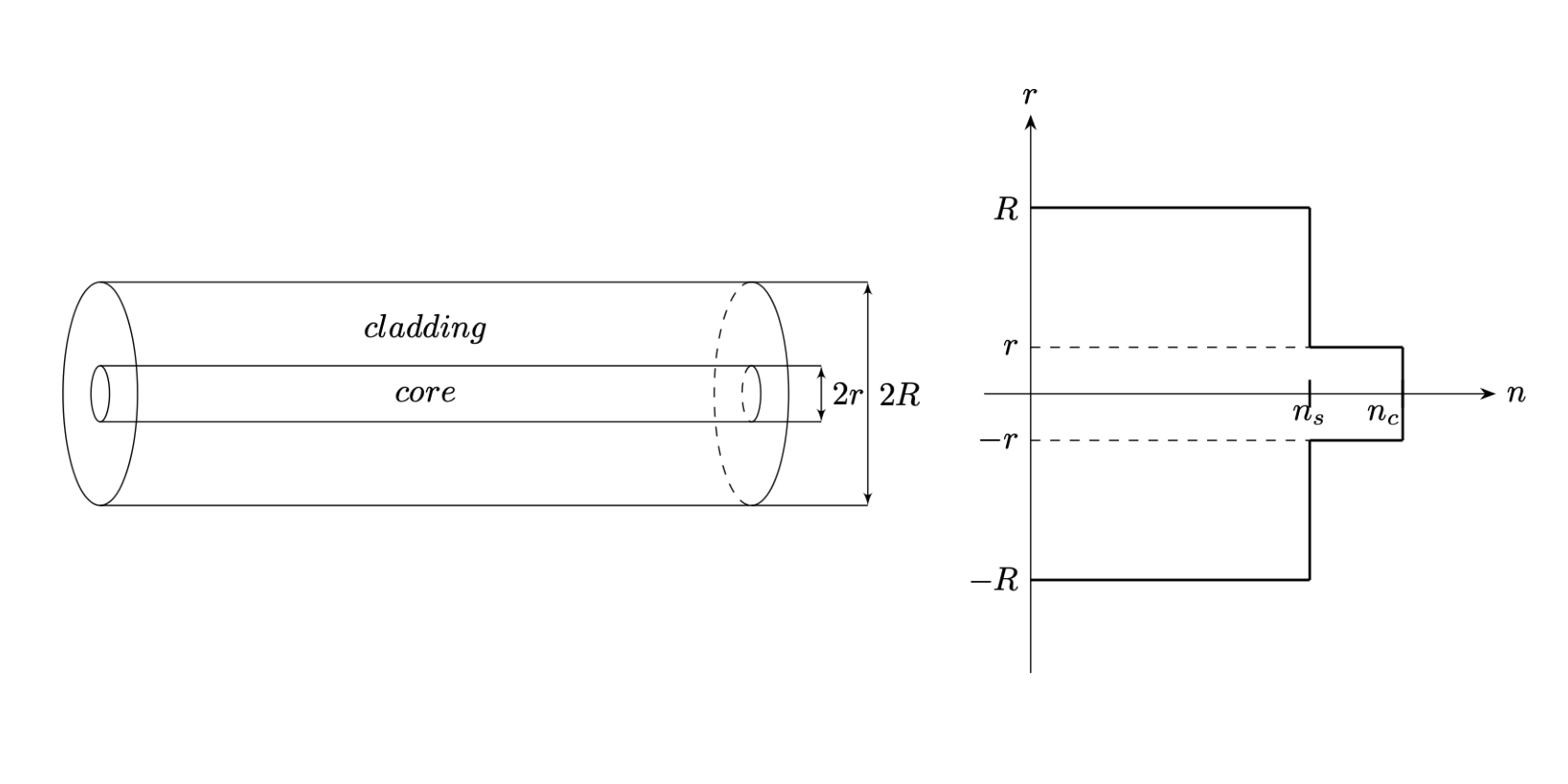
[Fig.1: Structure of an SMF optical fiber]
During the fiber manufacturing process, various optical structures can be embedded within the fiber, allowing them to be readily integrated into measurement and sensing systems. We consider a structure known as a Fiber Bragg Grating (FBG). In this configuration the fiber core contains defects with a period (shown in gray in figure 2), which are regions with a slightly increased refractive index.
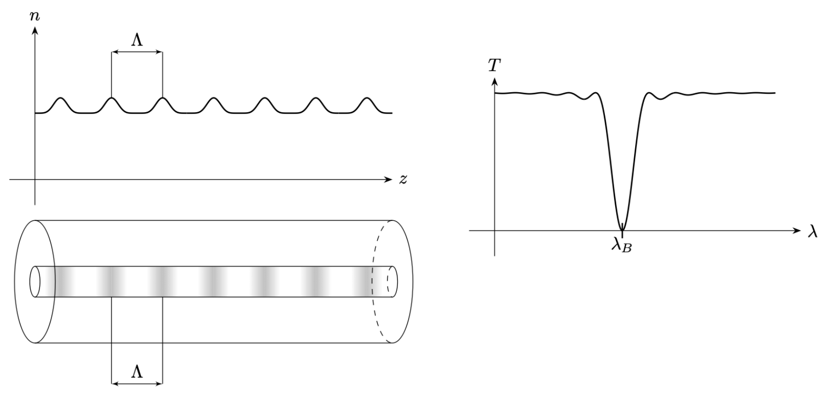
[Fig.2: Structure of an FBG]
A Fiber Bragg Grating exhibits the properties of a narrowband dielectric mirror: it reflects light whose vacuum wavelength is close to
Figure 2 shows the transmission spectrum of an FBG, i.e., the dependence of the energy transmission coefficient on the optical wavelength . The sharp minimum corresponds to the Bragg resonance at .
Instructions for using the FBG-Writer software
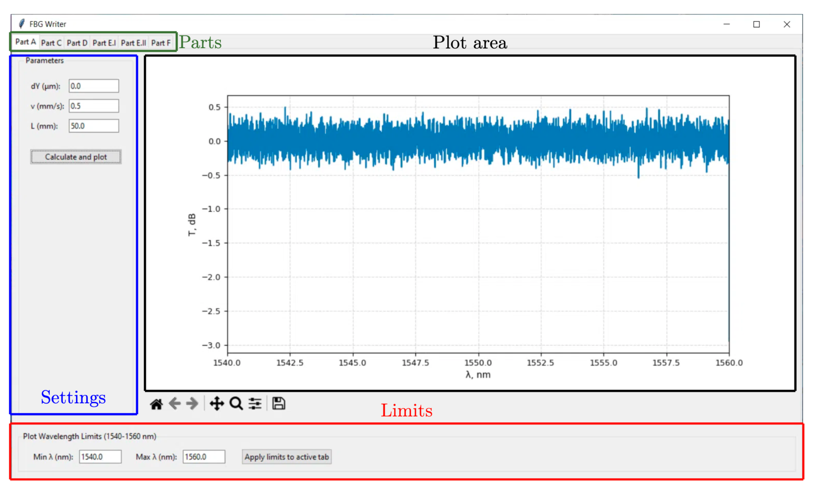
The software shown in figure 3 allows you to “fabricate” FBG and investigate their transmission spectra over the wavelength range . The plot of dependence is displayed in the “Plot area” after pressing the “Calculate and plot” button. The spectrometer shows the vacuum wavelength of light .
To get started with the software, select the tab corresponding to the desired part of the problem from the “Parts” menu. The parameter values can be adjusted in the “Settings” panel located on the left side of the application window. The wavelength range displayed on the plot is controlled by the “Min ” and “Max ” fields in the “Limits” panel. These limits can be set to any values within the interval . To apply the new limits, press the “Apply limits to active tab” button located in the “Limits” panel.
You can zoom in on the area on the graph. To do this, click on the button with a magnifying glass located on the toolbar below and select the area of interest on the graph. To return to the original scale, click on the button with the image of the house.
For convenience, throughout this problem the transmission coefficient is expressed in decibels (the conversion formula is ). In any practical measurement setup, there is a background illumination, so the value of cannot fall below a finite threshold.
Part A. FBG fabrication technology (5 т.)
One of the methods for manufacturing FBG involves drawing an optical fiber under a focused laser that emits very short but high-energy pulses of light.
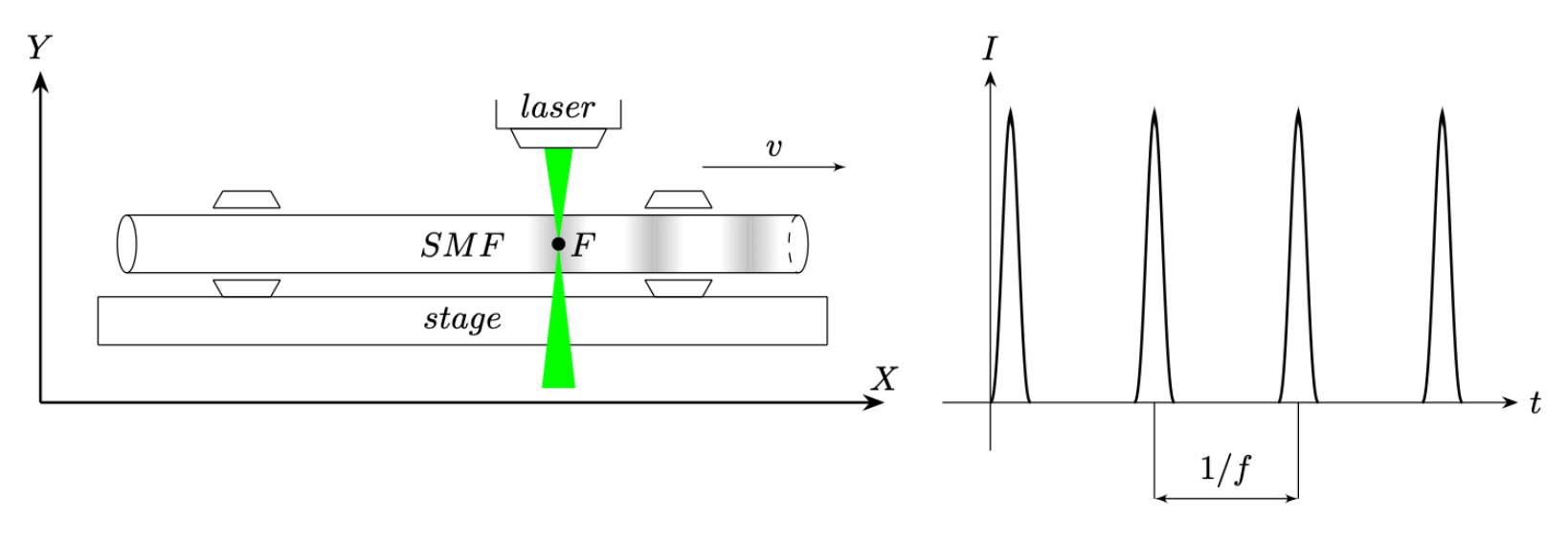
Let denote the frequency of pulses (see the graph of the dependence of the laser light intensity on time in figure 4), the fiber velocity is denoted by . The focused laser beam heats the fiber optic material and “sinters” it, forming small defects. If the velocity of the optical fiber is constant, then a periodic grating with a modulated refractive index is formed in it.
A.1 Express the defect period in terms of and .
. [0,2 т.]
Fiber Bragg Gratings are written using a pulsed laser with .
A.2 The refractive index of the fiber core material is . Estimate the fiber velocity that produces a grating with the wavelength of Bragg resonance .
. [0,4 т.]
For the FBG manufacturing, the scheme shown in figure 4 is used. A slightly stretched optical fiber is fixed in the stage. The fabrication is controlled using three parameters: , and . The manufacturing process and investigation of optical fiber include the following steps.
- The laser is off. Using , the vertical position of the fiber is adjusted. Ideally, the focused spot of the laser should coincide with the SMF center. If differs from the optimal value, then the grating is written with a lower refractive index modulation.
- The stage begins to “creep” along the axis and accelerates to the velocity .
- The laser turns on. The stage velocity is maintained constant and equal to .
- After the stage has passed the distance , the laser turns off and the stage stops.
- The transmission spectrum (the dependence of the energy transmission coefficient on the radiation wavelength ) of the resulting structure is measured.
To complete part A, open the “Part A” tab in the FBG-Writer program. The parameter is denoted as in the software.
A.3 Using , , write the grating. What is the wavelength of its Bragg resonance ?
. [0,2 т.]
A.4 Calculate the exact value of .
. [0,2 т.]
A.5 At what stage velocity will the wavelength be exactly ?
. [0,2 т.]
Now let us find the optimal parameter .
A.6 Write the gratings using , and different values of in the range . Plot the dependence of the transmission spectrum minimum on .
| () | (dB) |
|---|---|
[1,8 т.]
A.7 Determine the at which the strongest grating is written.
. [0,3 т.]
Let us study how the transmission spectrum minimum depends on the length of the grating .
A.8 Write the gratings using , and different values of . Plot the dependence of the transmission spectrum minimum on . Determine the slope of the linear section of the graph.
| (mm) | (dB) |
|---|---|
. [1,7 т.]
Part B. Coupled mode theory (2,9 т.)
The behavior of light inside the SMF can be approximately described using Coupled Mode Theory (CMT). Consider the propagation of radiation with the wavelength through the fiber core.
The total electric field inside the SMF can be expressed as the sum of two waves traveling in different directions:
where is the complex amplitude of the wave traveling in the positive direction of the fiber axis, and is the complex amplitude of the wave traveling in the negative direction of the fiber axis, is the magnitude of the wave vector.
When the radiation propagates in the SMF without any refractive index modulation, the amplitudes of both components remain constant:
However, when the radiation enters the grating, it begins to interact with its periodic structure. As a result, the amplitudes of the components change:
Here is the interaction constant, which is called the grating strength, is the derivative of the complex amplitude with respect to coordinate , is the derivative of the complex amplitude with respect to coordinate .
B.1 Eliminate the variable and obtain a second-order differential equation for . [0,5 т.]
Let us consider the problem of light passing through an FBG of length . A wave with amplitude falls on the grating on the left. A wave with amplitude emerges from FBG on the right. In this case, is the energy transmission coefficient.
B.2 Express in terms of and .
. [1,4 т.]
B.3 Determine the strength of the gratings written in question A8.
. [1 т.]
Part C. Calibration of an FBG temperature sensor (2,9 т.)
When the SMF is heated with the written FBG, the wavelength of the Bragg resonance changes. This is caused by the thermal expansion increasing the distance between adjacent defects and by the temperature-induced change in the refractive index. The wavelength shift of the Bragg resonance can be written as
where is the temperature change, is a constant with the units of .
Elongation of a sample with a length due to the thermal expansion is given by the equation , where is the temperature coefficient of expansion.
The temperature dependence of the refractive index is described by the equation , where is the refractive index change.
C.1 Derive the expression for in terms of , and .
. [0,4 т.]
To calibrate FBG as a temperature sensor, you have access to a grating with fixed parameters and a water bath with the ability to change the temperature in the range .
C.2 Open the “Part C” tab in the FBG-Writer program. Measure the dependence of the wavelength on .
| () | (nm) |
|---|---|
[1,2 т.]
C.3 Plot the dependence of on . Determine the value of the coefficient .
. [0,8 т.]
C.4 Estimate the minimum temperature change that can be detected using the FBG sensor. [0,5 т.]
Part D. Using the FBG temperature sensor (2,4 т.)
The FBG provided earlier was placed in a container with molten low-density polyethylene LDPE, which was kept in the air. The FBG transmission spectrum was measured once a minute. During this process the LDPE solidified.
D.1 Open the “Part D” tab in the FBG-Writer program. Measure the dependence of the wavelength on . Obtain the necessary data from the spectra and then calculate the dependence of temperature on time .
| (min) | (nm) | () |
|---|---|---|
[1,6 т.]
D.2 Plot the dependence of temperature on time . Determine the LDPE solidification temperature .
. [0,8 т.]
Part E. FBG dynamometer (3,9 т.)
When the SMF is stretched with the written FBG, the wavelength of the Bragg resonance changes. This is caused by the increase in spacing between adjacent defects and by the change in the refractive index of the sample due to elastic deformations of the medium. The change in the Bragg resonance wavelength induced by an applied force can be expressed as:
where is a constant with the units of . Fiber deformation is described by Hooke's law , where is the mechanical stress (measured in Pa), is the Young's modulus of the fiber material, is the strain ().
The dependence of the refractive index of medium on stretching is described by the equation , where is the refractive index change. Let denote the cross-sectional area of the fiber.
E.1 Derive the expression for in terms of , , and .
. [0,5 т.]
To calibrate the FBG as a strain sensor, you have access to a sample, one end of which is fixed, and a mechanical dynamometer that allows you to measure forces in the range . The end of the dynamometer spring is firmly connected to the free end of the fiber.
E.2 Open the “Part E.I” tab in the FBG-Writer program. Measure the dependence of the wavelength on .
| (mN) | (nm) |
|---|---|
[1 т.]
E.3 Plot the dependence of on . Determine the value of the coefficient .
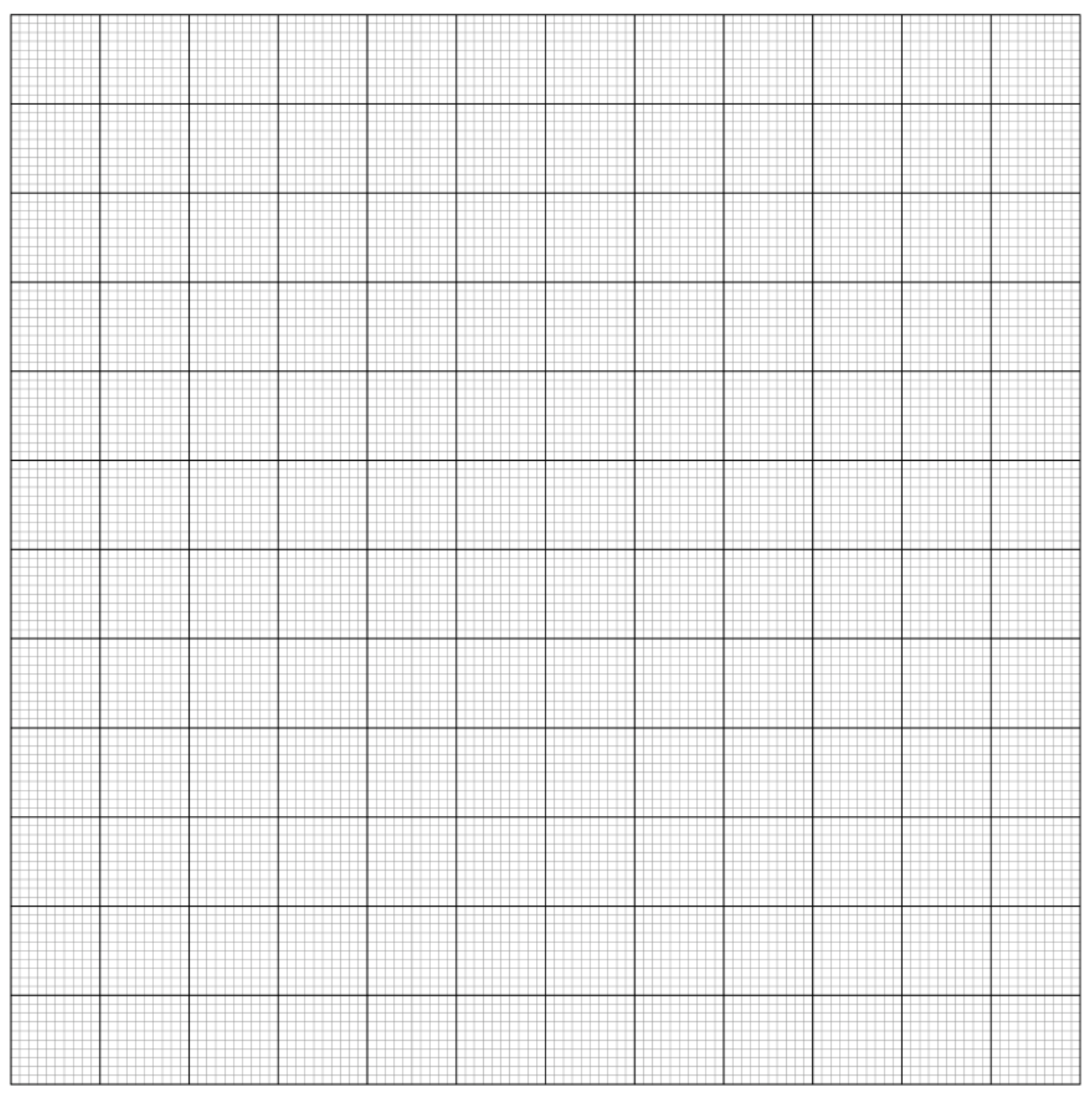
. [0,7 т.]
You are given a spring of unknown stiffness . One end of the SMF sample is fixed, and a spring is attached to the other end. The spring elongation is denoted as in the software.
E.4 Open the “Part E.II” tab in the FBG-Writer program. By changing the spring elongation in the range , measure the dependence and plot its graph. Determine the value of the spring stiffness .
| (mm) | (nm) |
|---|---|
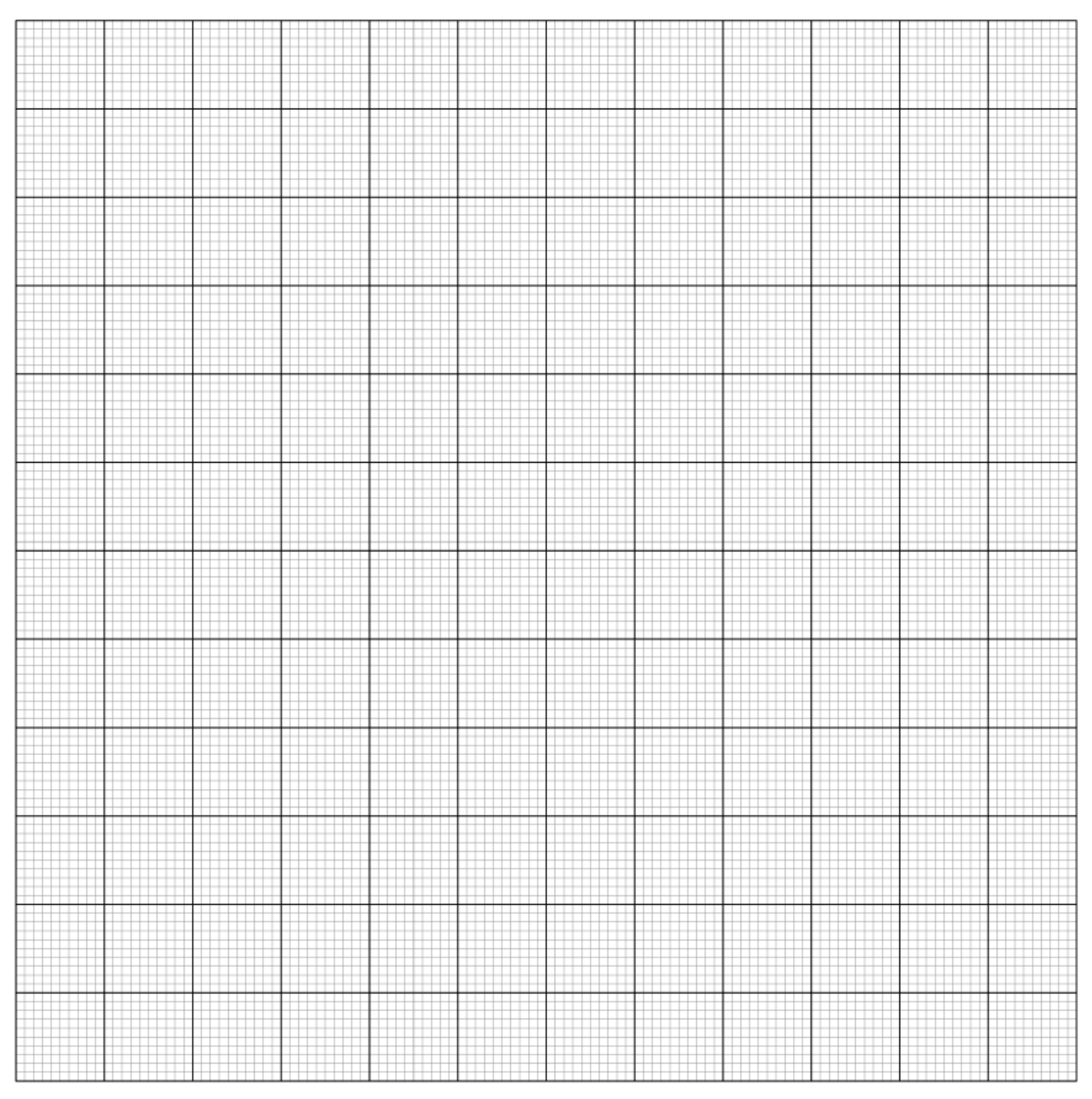
. [1,7 т.]
Part F. Birefringence in FBG (2,9 т.)
When an FBG is written using a femtosecond laser (pulse duration ), elongated defects are formed in it, which leads to effective birefringence. The strength of the grating and the wavelength of the Bragg resonance depend on the polarization of the light. For radiation with polarization directed along defects, we introduce and , and for radiation with perpendicular polarization — and (grating strength and wavelength, respectively). It is known that .
If an FBG is illuminated with polarized light, the observed transmission spectrum will depend on the angle between the polarization of the light and the orientation of the grating defects.
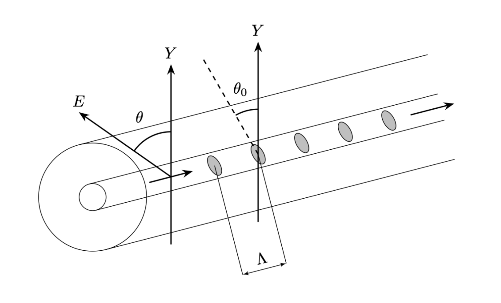
You are given a fixed grating with a length and birefringence. You can rotate the polarization of the radiation (angle in figure 5) and measure the transmission spectrum depending on the angle .
F.1 Open the “Part F” tab in the FBG-Writer program. Determine the angle at which the defects are oriented to the axis.
. [2 т.]
F.2 Find the values of , and , .
.
.
.
. [0,9 т.]
Решение
Внимание: Непълно решение
The archive solutions.txt explicitly lists the experimental solution as “E: (not available)”. The required FBG-Writer program and its generated measurement data are not included in the inspected 2026 archive inventory. The official blank answer sheets are preserved as question materials, not as solutions.
Оригинал в Архива: E.pdf · допълнителни данни: E_anssheet.pdf