Съдържание

Условие Experimental setup Отговори Решение

IZhO 2009, Експеримент — Задача 1. Air resistance force

Оригинал на условието (Word)Съобщи за грешка

Всички материали от IZhO 2009

V International Zhautykov Olimpiad — Experimental Competition, 17 January, 2009 · 17 януари 2009 г.

Please read the instructions first:

The Experimental part consists of one problem. This part of the competition lasts 3 hours.
Please only use the pen that will be given to you.
You can use your own non-programmable calculator for numerical calculations. If you don’t have one, please ask for it from Olympiad organizers.
You are provided with Writing sheet and additional papers. You can use the additional paper for drafts of your solutions but these papers will not be checked. Your final solutions which will be evaluated should be on the Writing sheets. Please use as little text as possible. You should mostly use equations, numbers, figures and plots.
Use only the front side of Writing sheets. Write only inside the bordered area.
Begin each question on a separate sheet.
Write on the blank writing sheets whatever you consider is required for the solution of the question.
Fill the boxes at the top of each sheet of paper with your country (Country), your student code (Student Code), the question number (Question Number), the progressive number of each sheet (Page Number), and the total number of Writing sheets (Total Number of Pages). If you use some blank Writing sheets for notes that you do not wish to be evaluated, put a large X across the entire sheet and do not include it in your numbering.
At the end of the exam, arrange all sheets for each problem in the following order:
- Used Writing sheets in order;
- The sheets you do not wish to be evaluated
- Unused sheets and the printed question.
Place the papers inside the envelope and leave everything on your desk. You are not allowed to take any paper or equipment out of the room

Условие

Air resistance force acting on a moving body depends on its velocity in a very complicated way. Different approximations are used to evaluate the air resistance force, such as

F = \beta_1 v, \qquad (1)

F = \beta_2 v^2, \qquad (2)

where $\beta_1$ , $\beta_2$ are some constants which depend on the size and form of the body, and $v$ stands for the speed of the body.

In this task you are asked to experimentally establish which of equations (1) or (2) describes better the air resistance force acting on the moving ball. To do so, you are asked to study the decaying pendulum oscillations in which balls are used as plummets.

Experimental setup

Equipment: tripod with a holder, thread, ruler, measuring tape, ping-pong ball, plasticine, sticky tape.

Attach the ball to the thread and fix the thread to the holder. Place the tripod at the edge of the desk so that the thread can freely hang down. Using the sticky tape provided, attach the ruler to the edge of the desk so that you can measure the deviation x. The point of suspension of the pendulum must be at the height of $h = 50\,cm$ above the ruler, the length of the thread from the point of suspension to the ball must be $L = 60cm$ .

Setup drawing: a vertical tripod rod of height h standing on a desk edge with a ruler; a thread of length L hangs from the labelled point of suspension at the top of the rod at angle φ to the vertical and passes the ruler at deviation x, ending in a ball below the desk. Labels: point of suspension, Tripod, φ, thread, h, L, x, ruler, ball.

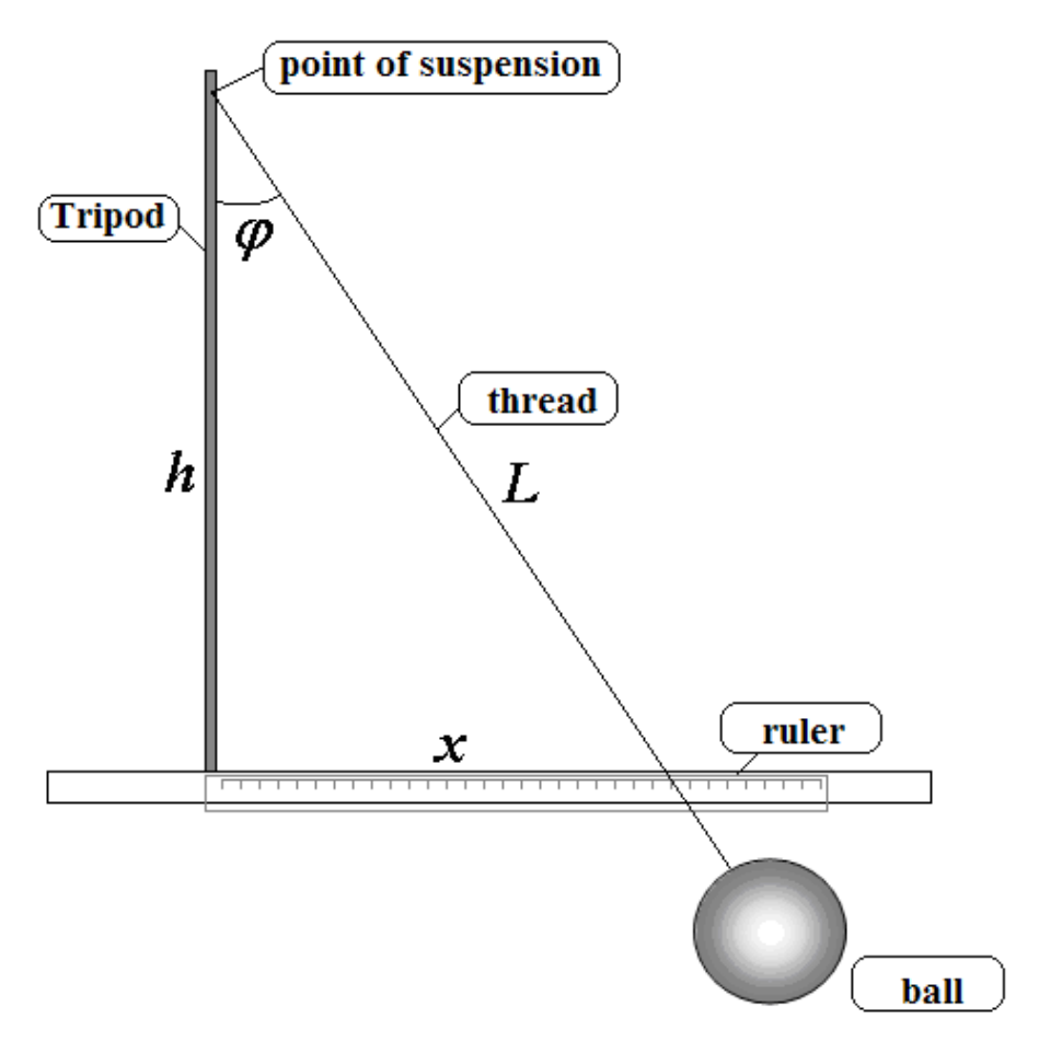
You will measure the following quantities:

$x$ is the deviation of the thread measured by the ruler;

$\varphi$ is the deviation angle.

Part 1. Energy loss during a single oscillation (9 points)

In this part use the ping-pong ball

1.1 Show that if the air resistance force depends on the body speed according to the law

F = \beta v^n,

then the loss of mechanical energy for one period equals

\Delta E = -CE_0^{\frac{n+1}{2}}, \qquad (3)

where $E_0$ is the initial mechanical energy of the ball, and $C$ is a certain constant. The saturation of oscillations is supposed to be weak. [1 т.]

1.2 Show that the mechanical energy $E$ of the ball at the maximal deviation is proportional to $(1 - \cos\varphi)$ .

In the following you should measure the energy of the ball in relative units. Assume that the potential energy of the ball is determined by

E = 1 - \cos\varphi. \qquad (4)

[1 т.]

1.3 Let $x_0$ be the initial deviation of the thread and let $x_1$ be the deviation of the thread after one period. Measure the dependence of $x_1$ on $x_0$ . Repeat the measurement of $x_1$ at least three times for each $x_0$ .

Using the data just obtained calculate the initial energy of the ball and the energy loss for one period. Write results of the measurements and calculations in Table 1. Plot the graph showing the dependence of the energy loss for one period on the initial energy of the ball $\Delta E(E_0)$ .

Table 1. Dependence of the energy loss on the initial energy.

$x_0$ , cm	$x_1$ , cm	$x_1$ , cm	$x_1$ , cm	$\langle x_1 \rangle$ , cm	$E_0$ , rel.units	$\Delta E$ ,rel. nits.

……. [3 т.]

1.4 Using equation (3) linearize the dependence $\Delta E(E_0)$ , i.e. find a transformation of variables

\xi = f_1(\Delta E), \quad \eta = f_2(E_0),

so that the dependence $\xi(\eta)$ becomes linear. Plot the graph $\xi(\eta)$ and determine the power $n$ in the dependence of air resistance force on the speed of the body. [3 т.]

1.5 State which of formulas (1) or (2) better fits the experimental data for the air resistance force. [1 т.]

Part 2. Saturation of oscillations, ping-pong ball (6 points)

In this part use the ping-pong ball provided.

One can show that if the air resistance force is described by equation (1), then the thread deviation after the k-th oscillation is described as

x_k = x_0 \lambda^k, \qquad (5)

where $\lambda$ is a constant. If the air resistance force is described by equation (2), then the saturation law has the form

x_k = \frac{x_0}{1 + Bx_0 k}, \qquad (6)

where $B$ is a constant.

2.1 Measure the dependence of the deviation $x_k$ on the number of oscillations $k$ at the fixed initial deviation $x_0 = 25\,cm$ . Write your results in Table 2.

Table 2. Saturation of oscillations of the ping-pong ball.

$k$	$x_k$ , cm	$x_k$ , cm	$x_k$ , cm
0	25	25	25
1
2
3

…. [2 т.]

2.2 Determine which of the saturation laws (5) or (6) fits the experimental data better. [3 т.]

2.3 Decide which of equations (1) or (2) describes the experimental situation better. [1 т.]

Part 3. Saturation of oscillations, plasticine ball (5 points)

In this part use the plasticine ball.

The oscillations of the pendulum with the plasticine ball saturate much slower, that is why it is hard to make a measurement after a single oscillation. Hence in this part you are asked to measure the number of oscillations $k$ which pass before the amplitude of oscillations decreases to the value $x_k$ .

3.1 Measure the number of oscillations $k$ after which the deviation of the ball decrease from the initial value $x_0 = 20\,cm$ till $x_k = 19, 18, \ldots, cm$ .

Put the results of the measurements into the Table 3. Plot the dependence of $x_k$ on the number of oscillations.

Table 3. Saturation of oscillations of the ping-pong ball.

$x_k$ , cm	$k$	$k$	$k$
20	0	0	0
19
18
17

…. [2 т.]

3.2 Determine which of the saturation laws (5) or (6) fits the experimental data better. [2 т.]

3.3 Decide which of equations (1) or (2) describes the experimental situation better. [1 т.]

Отговори

Решение

Solutions of the experimental problem

Part 1.

1.1 The power of energy losses equals

P = Fv = \beta v^{n+1},

therefore the energy loss during a single period can be represented as

\Delta E = \langle P \rangle T = \beta \langle v^{n+1} \rangle T = \beta T \left\langle (v_0 \sin \omega t)^{n+1} \right\rangle = \beta T v_0^{n+1} \left\langle (\sin \omega t)^{n+1} \right\rangle.

where $v_0$ - is the largest speed of the ball (assuming small damping). Energy of the ball is proportional to the square of the largest speed, $E_0 = \frac{mv_0^2}{2}$ . From here we obtain Eq. (3) of the problem set

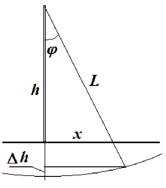
Pendulum diagram: vertical rod of height h, thread of length L at angle φ from the vertical, horizontal line with deviation x marked, an arc below showing the drop Δh of the ball.

\Delta E = -CE_0^{\frac{n+1}{2}}. \qquad (1)

1.2 At the point of maximal deviation the total mechanical energy equals only to the potential energy, thus

E = mgL(1 - \cos\varphi). \qquad (2)

1.3 The declination angle can be calculated using the equation

\varphi = \arcsin \frac{x}{\sqrt{x^2 + h^2}} \qquad (3)

Initial energy and its losses can be evaluated using equations

E_0 = 1 - \cos\varphi_0. \qquad (4)

\Delta E = \cos\varphi_1 - \cos\varphi_0. \qquad (5)

Results of measurements and calculations are shown in Table 1

Table 1.

$x_0$ , cm	$x_1$ , cm	$x_1$ , cm	$x_1$ , cm	$\langle x_1 \rangle$ , cm	$E_0$	$\Delta E$	$\ln E_0$	$\ln \Delta E$
25	20,6	20,7	20,5	20,6	0,1092	0,0311	-2,21	-3,47
24	20,0	19,5	20,5	20,0	0,1019	0,0278	-2,28	-3,58
23	19,0	19,0	19,5	19,2	0,0948	0,0261	-2,36	-3,65
22	18,0	18,5	18,6	18,4	0,0877	0,0241	-2,43	-3,73
21	17,5	17,6	17,8	17,6	0,0809	0,0218	-2,52	-3,83
20	17,0	17,1	17,1	17,1	0,0742	0,0185	-2,60	-3,99
19	16,6	16,5	16,6	16,6	0,0676	0,0150	-2,69	-4,20
18	15,6	15,4	15,5	15,5	0,0613	0,0148	-2,79	-4,22
17	15,0	14,9	14,8	14,9	0,0552	0,0120	-2,90	-4,42
16	14,0	14,2	14,2	14,1	0,0494	0,0102	-3,01	-4,58
15	13,5	13,3	13,5	13,4	0,0438	0,0082	-3,13	-4,80
14	12,6	12,4	12,6	12,5	0,0385	0,0073	-3,26	-4,92
13	11,8	11,5	11,6	11,6	0,0334	0,0064	-3,40	-5,05
12	10,7	10,7	10,7	10,7	0,0287	0,0057	-3,55	-5,17
11	10,0	9,8	9,9	9,9	0,0243	0,0045	-3,72	-5,41
10	9,2	9,3	9,3	9,3	0,0202	0,0028	-3,90	-5,89
9	8,2	8,0	8,3	8,2	0,0165	0,0028	-4,11	-5,86
8	7,5	7,4	7,3	7,4	0,0131	0,0019	-4,34	-6,29

Plot of the energy losses with respect to initial energy is shown in Fig. 1.

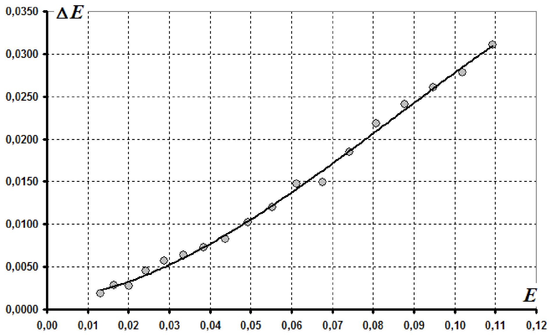
Graph of ΔE (vertical axis, 0,0000 to 0,0350) against E (horizontal axis, 0,00 to 0,12): measured points with a smooth upward-curving fitted line from about (0,013; 0,002) to (0,11; 0,031). — Рис. 1

4 Experimentally obtained curve looks similar to a power law. To determine the power it is most convenient to use a double logarithmic scale,

\ln|\Delta E| = \ln C + \frac{n+1}{2} \ln E_0, \qquad (6)

such that the tangent is related to the exponent. Logarithms of measured parameters are also shown in Table 1. The plot of the required dependence in the double logarithmic scale is shown in Fig. 2. Tangent of this plot is approximately equal to $\frac{n+1}{2} \approx 1{,}35$ , which leads to $n \approx 1{,}7$ .

Double-logarithmic plot: horizontal scale from -5,0 to -2,0 labelled ln E at the top, vertical scale from -3,0 to -7,0 on the right labelled ln ΔE; diamond data points lie along a straight line from about (-4,3; -6,3) to (-2,2; -3,5). — Рис. 2

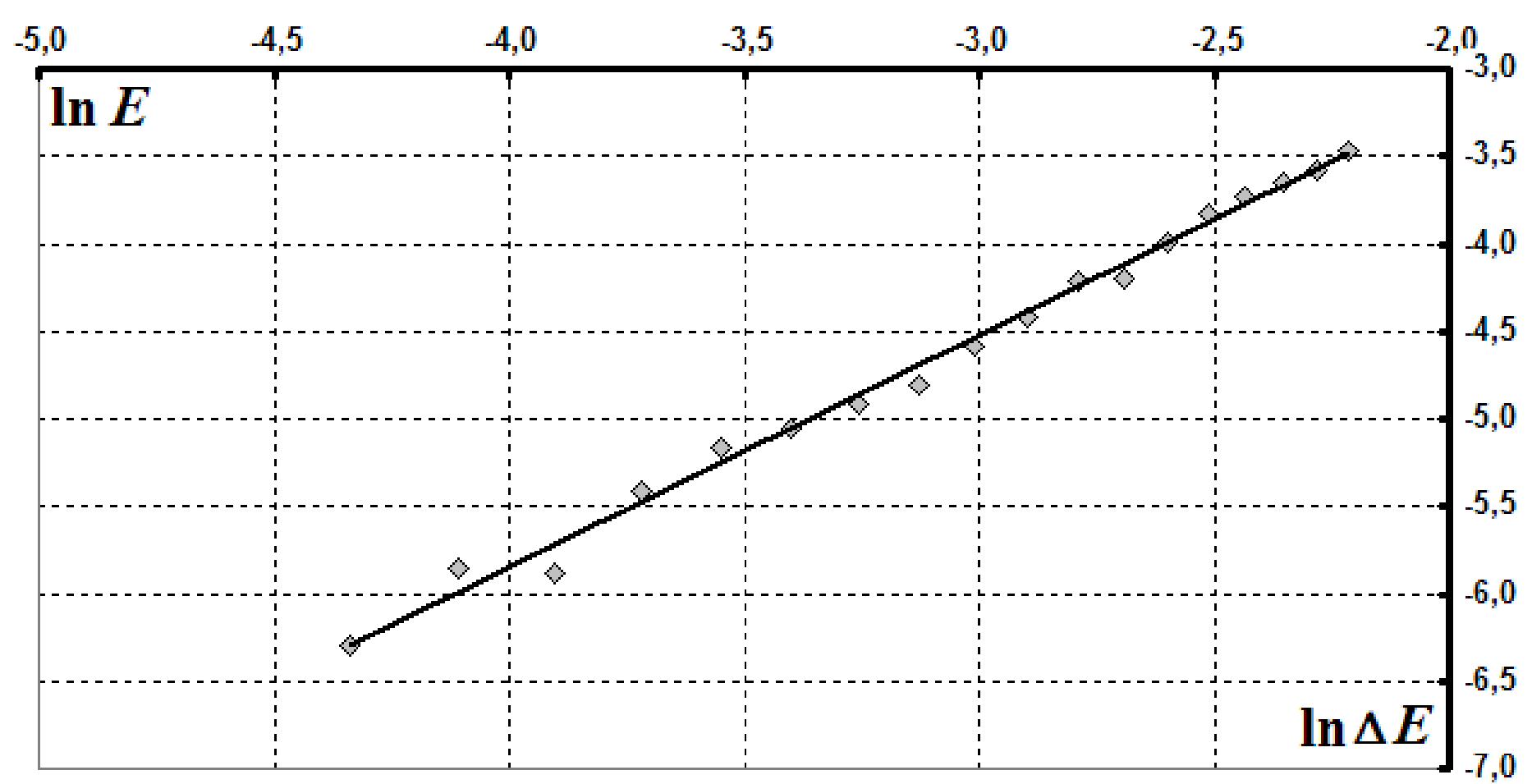
1.5 Obtained exponent is closer to 2, so Eq.(2) describes the experimental data better than eq.(1).

Part 2.

2.1 Results of the measurements are shown in Fig. 2.

Table 2.

$k$	$x_k$ , cm	$x_k$ , cm	$x_k$ , cm	$\langle x_k \rangle$ , cm	$\frac{1}{\langle x_k \rangle}$	$\ln \langle x_k \rangle$
0	25,0	25,0	25,0	25,0	0,040	3,219
1	22,0	21,0	21,0	21,3	0,047	3,060
2	18,0	17,5	17,7	17,7	0,056	2,875
3	15,5	16,0	15,5	15,7	0,064	2,752
4	13,5	13,6	13,3	13,5	0,074	2,600
5	11,5	12,0	12,0	11,8	0,085	2,471
6	10,5	11,0	10,7	10,7	0,093	2,373
7	10,0	9,6	9,8	9,8	0,102	2,282
8	9,5	9,0	8,8	9,1	0,110	2,208
9	8,5	8,3	7,5	8,1	0,123	2,092
10	7,5	7,5	7,0	7,3	0,136	1,992
11	7,0	7,0	6,5	6,8	0,146	1,922

2.2 To check equations (5)-(6) it is necessary to plot the dependences of $\ln\langle x_k \rangle$ (Fig. 3) and $\frac{1}{\langle x_k \rangle}$ (Fig. 4) on the number of oscillations $k$ .

Graph of ln⟨x_k⟩ (vertical axis, 1,5 to 3,5) against k (0 to 12): diamond points on a slightly concave decreasing curve from 3,22 at k = 0 to 1,92 at k = 11. — Рис. 3

Graph of 1/⟨x_k⟩ (vertical axis, 0,00 to 0,16) against k (0 to 12): diamond points close to a straight rising line from 0,04 at k = 0 to about 0,145 at k = 11. — Рис. 4

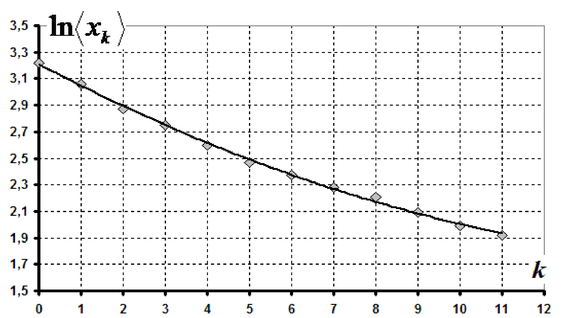
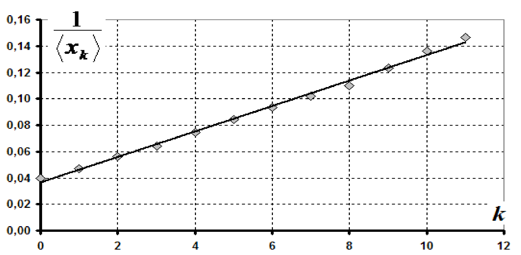
Dependence of $\frac{1}{\langle x_k \rangle}$ on $k$ is closer to linear, therefore, equation (6) describes experimental data

2.3 Since equation (6) follows from the quadratic dependence of the air resistance force on velocity, then the experimental data supports equation (2).

Part 3.

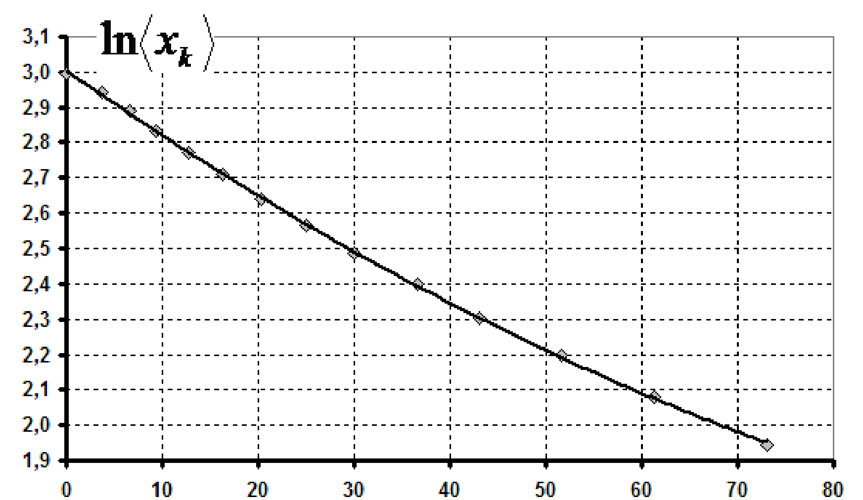
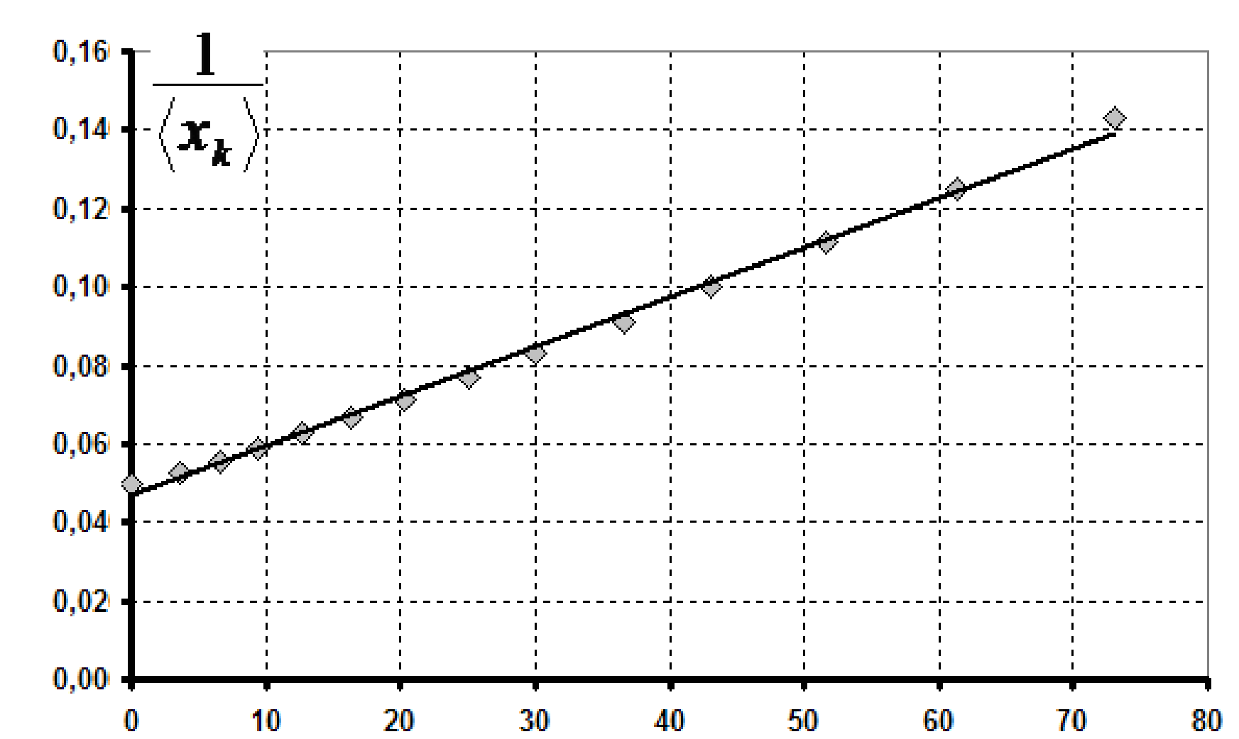
3.1 Results of measurement are shown in Table 3. The processing of the data follows the steps of Part 2.

$x_k$ , cm	$k$	$k$	$k$	$\langle k \rangle$	$\frac{1}{\langle x_k \rangle}$	$\ln \langle x_k \rangle$
20	0	0	0	0,0	0,050	2,996
19	4	4	3	3,7	0,053	2,944
18	7	7	6	6,7	0,056	2,890
17	10	10	8	9,3	0,059	2,833
16	13	13	12	12,7	0,063	2,773
15	16	17	16	16,3	0,067	2,708
14	21	21	19	20,3	0,071	2,639
13	25	25	25	25,0	0,077	2,565
12	30	30	30	30,0	0,083	2,485
11	37	36	37	36,7	0,091	2,398
10	43	43	43	43,0	0,100	2,303
9	52	51	52	51,7	0,111	2,197
8	62	61	61	61,3	0,125	2,079
7	74	72	73	73,0	0,143	1,946

3.2 Графики зависимостей $\ln\langle x_k \rangle$ (рис. 5) и $\frac{1}{\langle x_k \rangle}$ (рис. 6) от числа колебаний $k$ показывают, что и в данном случае формула (6) точнее описывает экспериментальные данные.

3.3 In this case quadratic dependence also describes the experimental situation better.

Marking scheme.

Item	Content	Points
1.1	- loss power	0,5
	- energy-velocity relation	0,5
1.2	- expression for the potential energy	1,0
1.3	Measurements:
	- measurement range $x_0$ (from 25 to 10 cm);	0,5
	- not less than 10 points;	0,5
	Evaluation of $E_0$ and $\Delta E$ for all points;	1
	Plot (axes are signed and numbered, dots are plotted, smoothing curve is indicated)	1
1.4	Double logarithmic scale (or other linearization);	1
	Evaluation of logarithms;	0,5
	Plot (axes are signed and numbered, dots are plotted, smoothing curve is indicated);	0,5
	Determination of the exponent (using all points)	1
1.5	Substantiated conclusion on the applicability of equation (2)	1
2.1	Measurements
	- not less than 10 points;	1,5
	- averaging;	0,5
2.2	Data processing to check to dependences:
	- linearization;	0,5+0,5
	- Plots of linearized curves;	0,5+0,5
	- Conclusion on the applicability of equation (2)	1
2.3	Substantiated conclusion on the applicability of equation (2)	1
3.1	Measurements:
	- range from 20 cm to 10 cm;	0,5
	- not less than 10 points;	0,5
	Plot (axes are signed and numbered, dots are plotted, smoothing curve is indicated)	1
3.2	- Plots of linearized curves;	1
	- conclusion on the applicability of Eq. (6)	1
3.3	Substantiated conclusion on the applicability of equation (2)	1

Graph of ln⟨x_k⟩ (vertical axis, 1,9 to 3,1) against k (0 to 80) for the plasticine ball: diamond points on a slightly curved decreasing line from 3,0 at k = 0 to about 1,95 at k = 73. — Рис.5

Graph of 1/⟨x_k⟩ (vertical axis, 0,00 to 0,16) against k (0 to 80) for the plasticine ball: diamond points along a straight rising line from 0,05 at k = 0 to about 0,14 at k = 73. — Рис.6

Оригинал в Архива: IZhO-2009-Exp_eng.doc · официални решения: IZhO-2009-Exp_eng_sol.doc