Съдържание

IZhO 2020, Експеримент — Задача 1. Maxwell’s Disc

Оригинал на условието (PDF)Съобщи за грешка

Всички материали от IZhO 2020

XVI International Zhautykov Olimpiad/Experimental Competition — EXPERIMENTAL COMPETITION, 11 January, 2020 · 11 януари 2020 г. · 15 т.

Please read the instructions first:

The Experimental competition consists of one problem. This part of the competition lasts 3 hours.
Please only use the pen that is provided to you.
You can use your own non-programmable calculator for numerical calculations. If you don’t have one, please ask for it from Olympiad organizers.
You are provided with Writing sheet and additional papers. You can use the additional paper for drafts of your solutions but these papers will not be checked. Your final solutions which will be evaluated should be on the Writing sheets. Please use as little text as possible. You should mostly use equations, numbers, figures and plots.
Use only the front side of Writing sheets. Write only inside the bordered area.
Fill the boxes at the top of each sheet of paper with your country (Country), your student code (Student Code), the question number (Question Number), the progressive number of each sheet (Page Number), and the total number of Writing sheets (Total Number of Pages). If you use some blank Writing sheets for notes that you do not wish to be evaluated, put a large X across the entire sheet and do not include it in your numbering.
At the end of the exam, arrange all sheets for each problem in the following order:
- Used Writing sheets in order.
- The sheets you do not wish to be evaluated.
- Unused sheets.
- The printed problems.
Place the papers inside the envelope and leave everything on your desk. You are not allowed to take any paper or equipment out of the room

Условие

In this experiment, you are asked to design all the experimental setups by yourself, connect threads and mark them up if necessary. You can further fasten the discs with pieces of plasticine.

Instruments and equipment: Maxwell's disk (two disks mounted on a wooden stick), two tripods, threads, a wooden stick, stopwatch, ruler, 2 loads of 100 g each, a piece of plasticine, adhesive tape.

Do not calculate experimental errors if you are not asked to do so.

Part 1. Rolling down

Pull two threads between the two tripods, so that they are parallel to each other and make up some angle $\alpha$ to the horizontal. Maxwell's disc should slide without slipping on these threads, resting on the wooden parts of the stick.

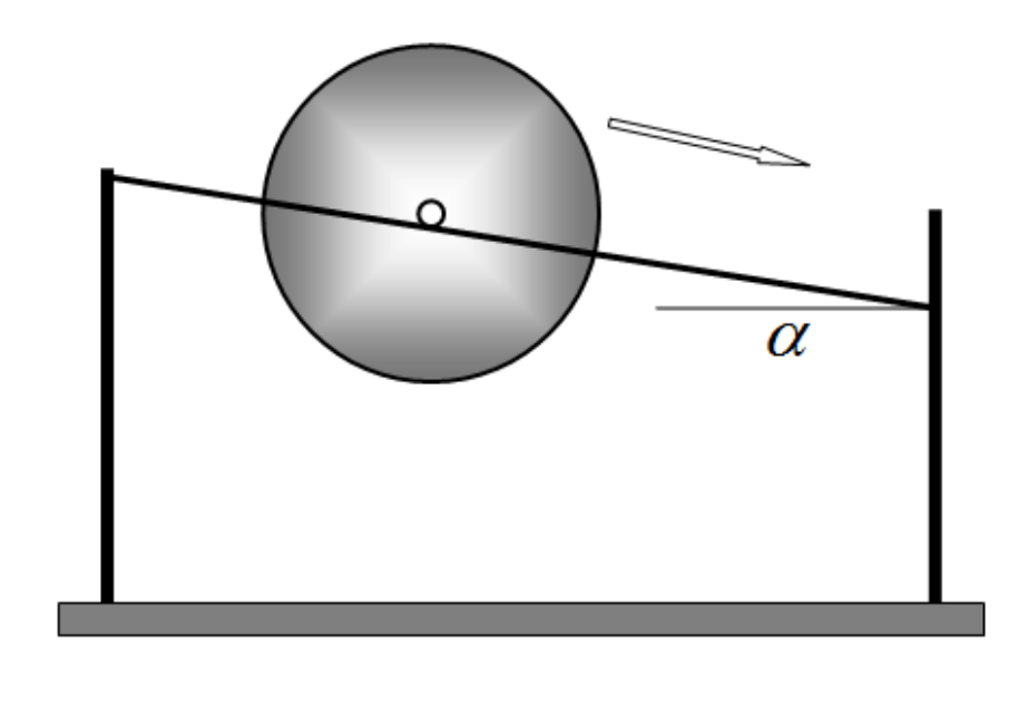
A disc on an axis resting on an inclined thread stretched between two vertical posts on a base; an arrow shows the direction of rolling down the slope; the angle α between the thread and the horizontal is marked at the lower right post.

1.1 Derive the formula for the acceleration with which the axis of the disk rolls, depending on the angle of inclination $\alpha$ . Assume the disc is homogeneous and neglect the mass of the wooden stick.

1.2 Investigate experimentally the law of motion, i.e. the dependence of the coordinate of the axis of the disk $x(t)$ along the thread on time $t$ , when it rolls along the threads. Draw a graph of the resulting dependence. Prove that the motion of the disc axis is approximately uniformly accelerated. Calculate the disk axis acceleration. Indicate at what angle you have taken your measurements.

1.3 Measure the dependence of the acceleration of the disk axis on the angle of inclination of the threads $\alpha$ . Draw a graph of the resulting dependence.

1.4 On the same graph plot the theoretical dependence of the acceleration on the angle of inclination $\alpha$ of the threads. Indicate the results of additional measurements that you have used to calculate the accelerations.

Part 2. Moving down

Hang the disc on two threads as shown. Fix the threads on the stick with the adhesive tape to prevent them from slipping. Wind the threads onto the sticks and release the disc.

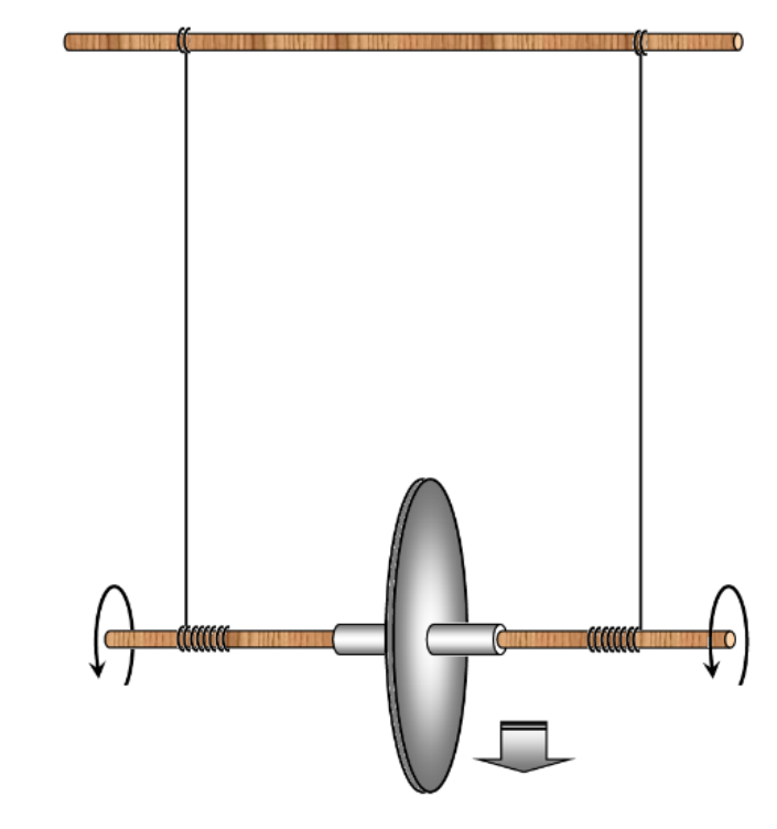
Maxwell's disc on a horizontal stick hanging on two vertical threads from a fixed horizontal rod; the threads are wound on the stick on both sides of the disc, curved arrows show the rotation of the stick ends, and an arrow below the disc points down.

2.1 Investigate the law of motion of the disk axis when it moves down. Draw a graph of the resulting dependence.

2.2 According to the measurement data, calculate the acceleration at which the axis of the disc moves down. Estimate the experimental error of the obtained acceleration.

2.3 Derive the theoretical formula for the acceleration of the disc axis. Calculate the theoretical value of the acceleration with which the axis of the disc moves down.

Part 3. Moving up

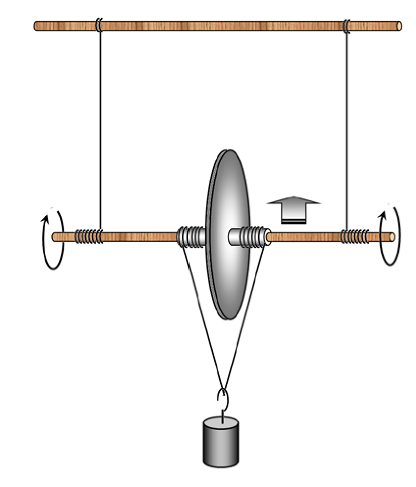
Maxwell's disc hanging on two vertical threads from a fixed horizontal rod; two additional threads wound on the stick next to the disc form a V and hold a suspended cylindrical load on a hook; curved arrows show the rotation of the stick ends and an arrow above the disc points up.

If two additional threads are wound on the stick and a load is suspended on them, then with proper winding of the threads, the disk starts to move up.

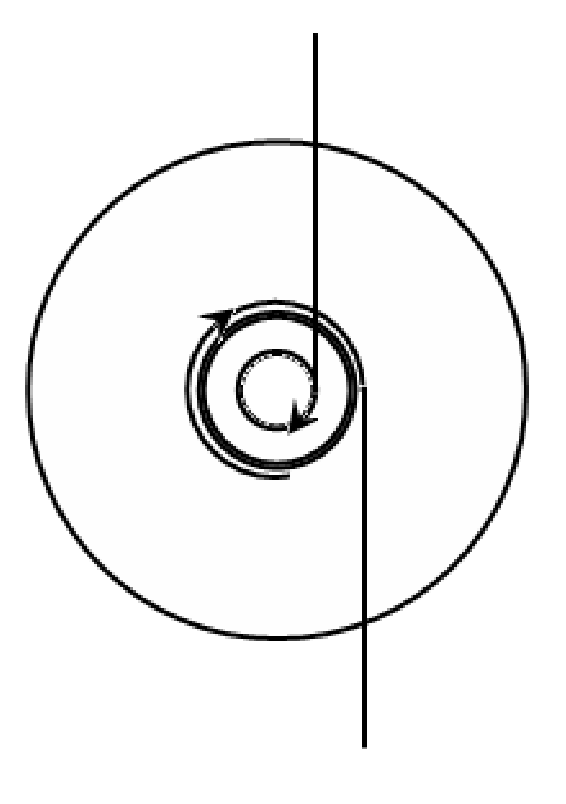
3.1 Design the experimental setup such that the disk moves up spinning around. Show schematically in the figure how the threads should be wound on the stick.

3.2 Measure the dependence of the acceleration of the disk axis for different masses of suspended loads.

Отговори

Решение

SOLUTION TO THE EXPERIMENTAL COMPETITION

Maxwell’s disk (15,0 points)

Part 1. Rolling down

1.1 The basic equation of the dynamics of rotational motion relative to the point of contact of the stick and thread is written as

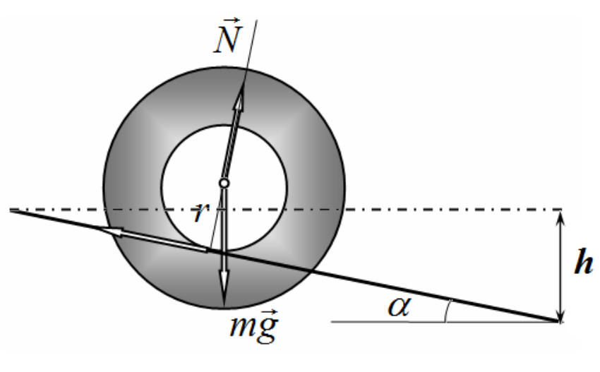
Cross-section of the disc (grey ring) with the stick of radius r at its centre resting on an inclined thread; forces N (up along the contact normal) and mg (down) are drawn from the centre; the angle α between the thread and the horizontal and the height h are marked on the right.

\left(\frac{mR^2}{2} + mr^2\right)\frac{a}{r} = mgr\sin\alpha, \qquad (1)

where $R$ stands for the disc radius and $r$ denotes the stick radius.

The formula for the disc axis acceleration is thus obtained as

a = \frac{g}{1+\frac{1}{2}\left(\frac{R}{r}\right)^2}\sin\alpha. \qquad (2)

1.2 To change and measure the angle that the threads make with the horizontal, it is necessary to shift up one of the holders of the tripod to the height $h$ . Therefore, the sine of the inclination angle is found as

\sin\alpha = \frac{h}{L}, \qquad (3)

where $L$ designates the threads’ length (in our experiment $L = 70sm$ ).

In this part, the measurements have been taken for $h = 3{,}0sm$ . It is necessary to put marks on the threads at regular intervals and fix the travel time with a stopwatch. The difficulty is that in practice it is difficult to release the disk from the first mark without an initial push, therefore the first mark is used as a reference point, but the disk speed is thus not zero! The time dependence of the disc axis position is shown in Table 1 and in Fig. 1.

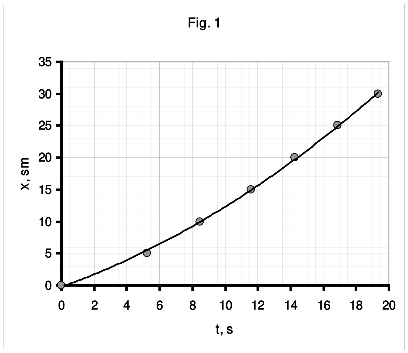
Table 1.

x. см	t, c	x/t
0	0
5	5,24	0,95
10	8,44	1,18
15	11,57	1,30
20	14,25	1,40
25	16,90	1,48
30	19,34	1,55

The law of uniform acceleration has the form

x(t) = v_0 t + \frac{at^2}{2}. \qquad (4)

Various methods can be used for linearization, but the following is preferred:

\frac{x}{t} = v_0 + \frac{a}{2}t. \qquad (5)

Fig. 2 shows a plot of the value $\frac{x}{t}$ (actually, average speed) versus time $t$ .

Fig. 2: graph of x/t, sm/s (0,00 to 2,00) versus t, s (0 to 20) with five points between t ≈ 8,4 s and 19,3 s lying on a straight line rising from about 1,18 to 1,55.

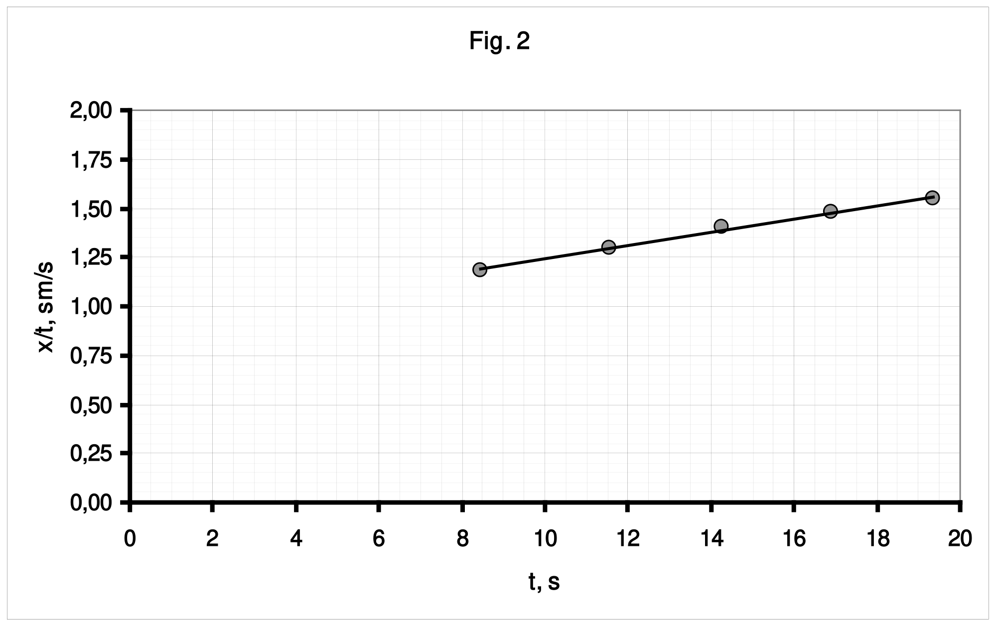
The approximate linearity of this dependence proves that the experimental law of motion can be described by function (4).

The acceleration of the disk axis is equal to twice the value of the slope of this graph and it is evaluated by the method of least squares to be equal to

a = 0{,}081\frac{sm}{s^2}. \qquad (6)

1.3 Similar measurements have to be carried out for other values of the inclination angles of the threads. The corresponding results are shown in Table 2.

Table 2

h=5 sm			h=7 sm			h=9 sm			h=11 sm
x. sm	t, s	x/t	x. sm	t, s	x/t	x. sm	t, s	x/t	x. sm	t, s	x/t
0			0			0			0
5	4,66	1,07	5	3,53	1,42	5	3,30	1,52	5	3,38	1,48
10	7,51	1,33	10	5,81	1,72	10	5,24	1,91	10	5,32	1,88
15	9,95	1,51	15	7,94	1,89	15	7,14	2,10	15	6,92	2,17
20	12,28	1,63	20	9,70	2,06	20	8,73	2,29	20	8,36	2,39
25	14,23	1,76	25	11,26	2,22	25	10,10	2,48	25	9,45	2,65
30	16,10	1,86	30	12,84	2,34	30	11,46	2,62	30	10,89	2,75

Figure 3 shows the graphs of the dependences $\frac{x}{t}$ on time $t$ which are used to calculate the experimental values of the accelerations.

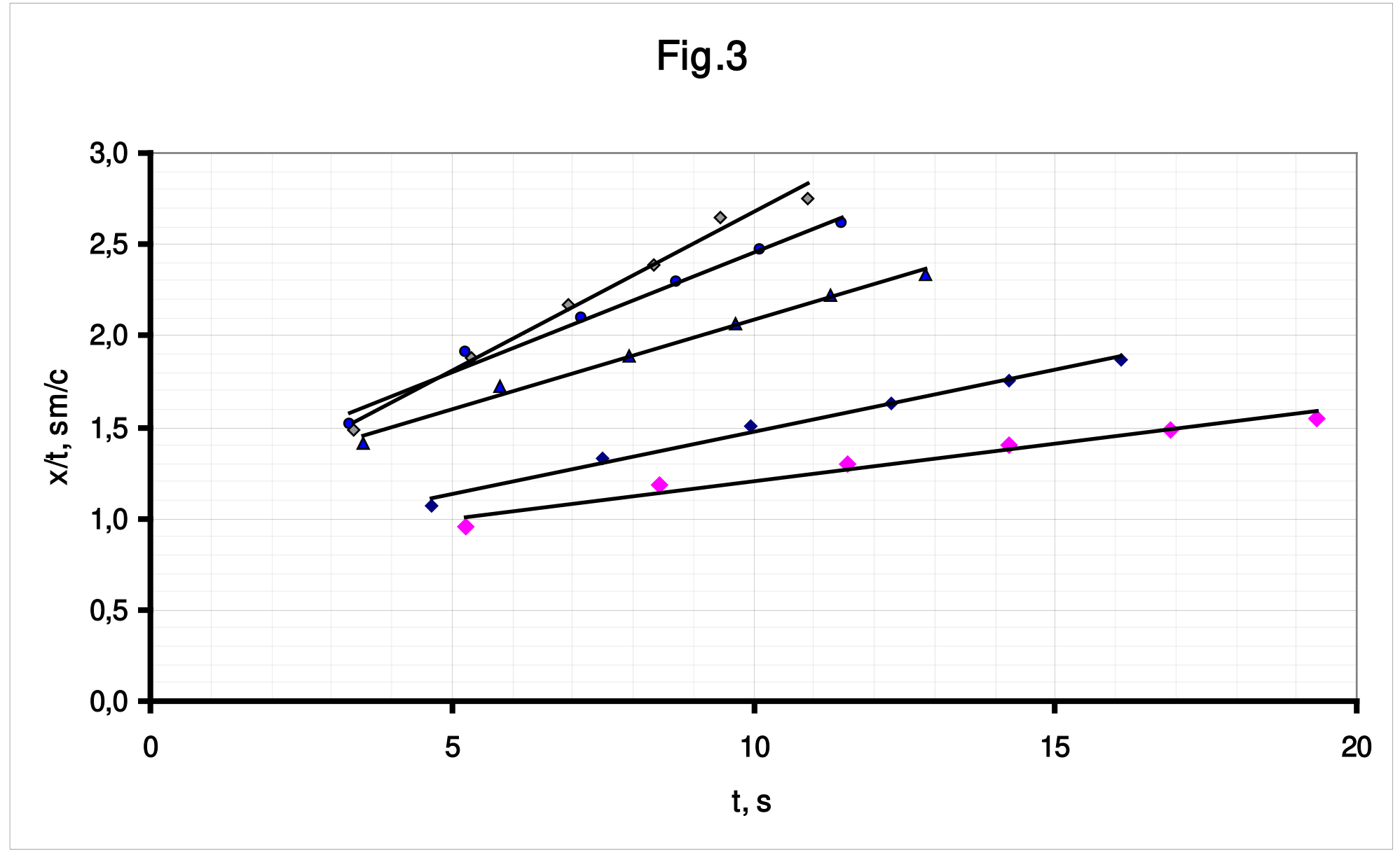
Fig.3: graph of x/t, sm/c (0,0 to 3,0) versus t, s (0 to 20) with five data series (different markers) from Tables 1 and 2, each fitted by a straight line; steeper lines correspond to larger h.

Table 3 shows the accelerations calculated by the slope coefficients of the graphs and corresponding theoretical values evaluated via formula (2). In the calculations, the following measured values are taken: the disk diameter $D = 85mm$ and the stick diameter $d = 3{,}0mm$ . Fig. 4 shows graphs of the dependences of the accelerations on the angle of threads inclination.

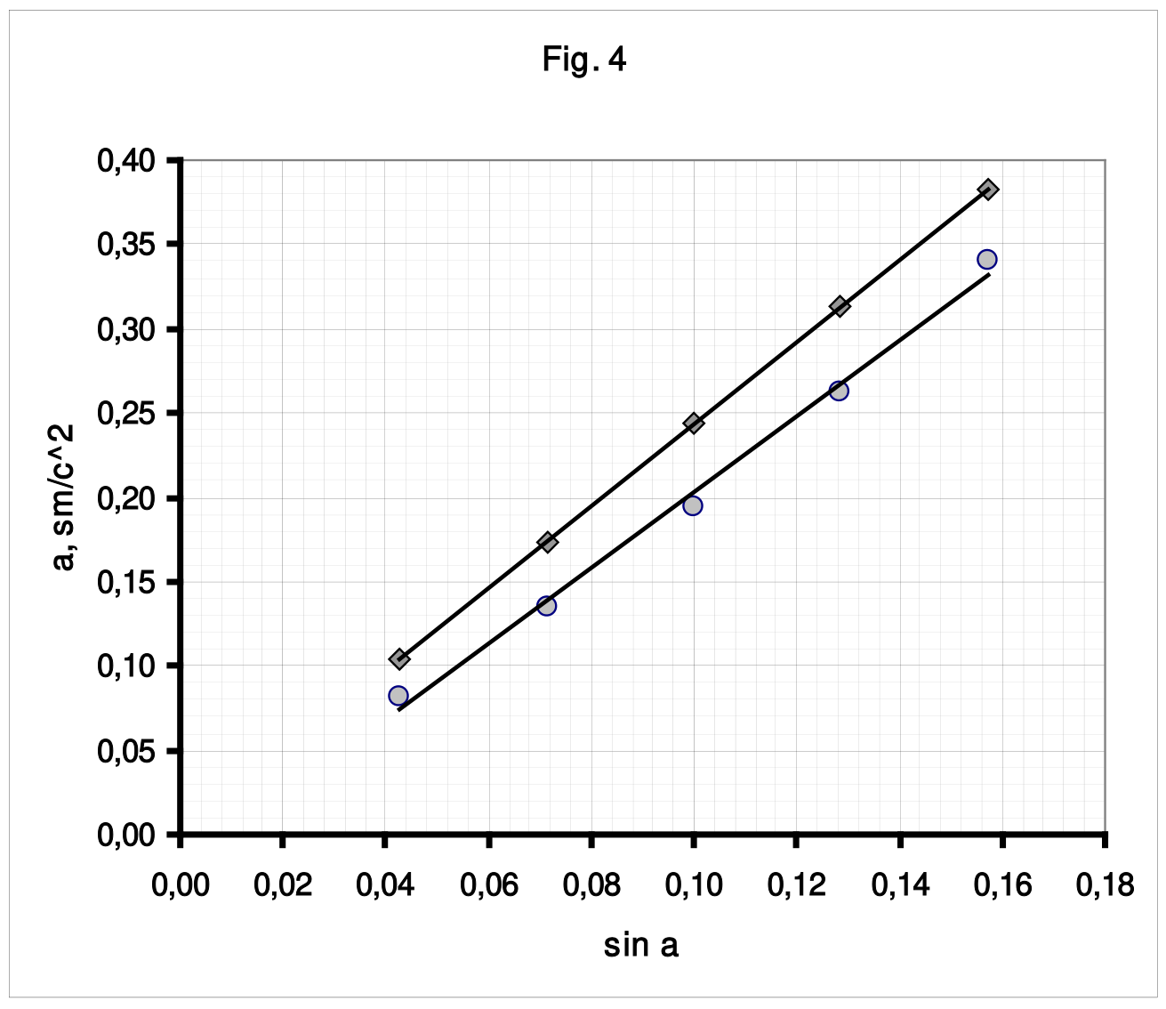
Fig. 4: graph of a, sm/c^2 (0,00 to 0,40) versus sin a (0,00 to 0,18) with two straight lines: theoretical values (diamonds, upper line) and experimental values (circles, lower line) for sin α = 0,043…0,157.

Table 3

h , sm	а, theor. sm/s²	а, exper. sm/s²	$\sin\alpha$
3	0,104	0,081	0,043
5	0,174	0,135	0,071
7	0,244	0,195	0,100
9	0,313	0,262	0,129
11	0,383	0,340	0,157

Part 2. Moving down

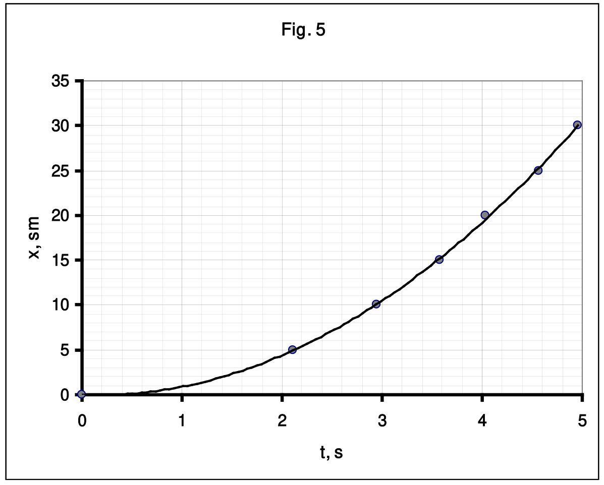
2.1 In this case, the travel time is small, therefore, measurements should be carried out for each coordinate repeatedly. Table 4 lists the results of the time measurements needed for the disc to travel distance $x$ , averaged over 3 measurements. Fig. 5 demonstrates a graph of the obtained dependence.

Table 4.

x, sm	t, s	x/t	t²
0	0		0
5	2,11	2,37	4,45
10	2,95	3,39	8,70
15	3,58	4,19	12,82
20	4,03	4,96	16,24
25	4,56	5,48	20,79
30	4,96	6,05	24,60

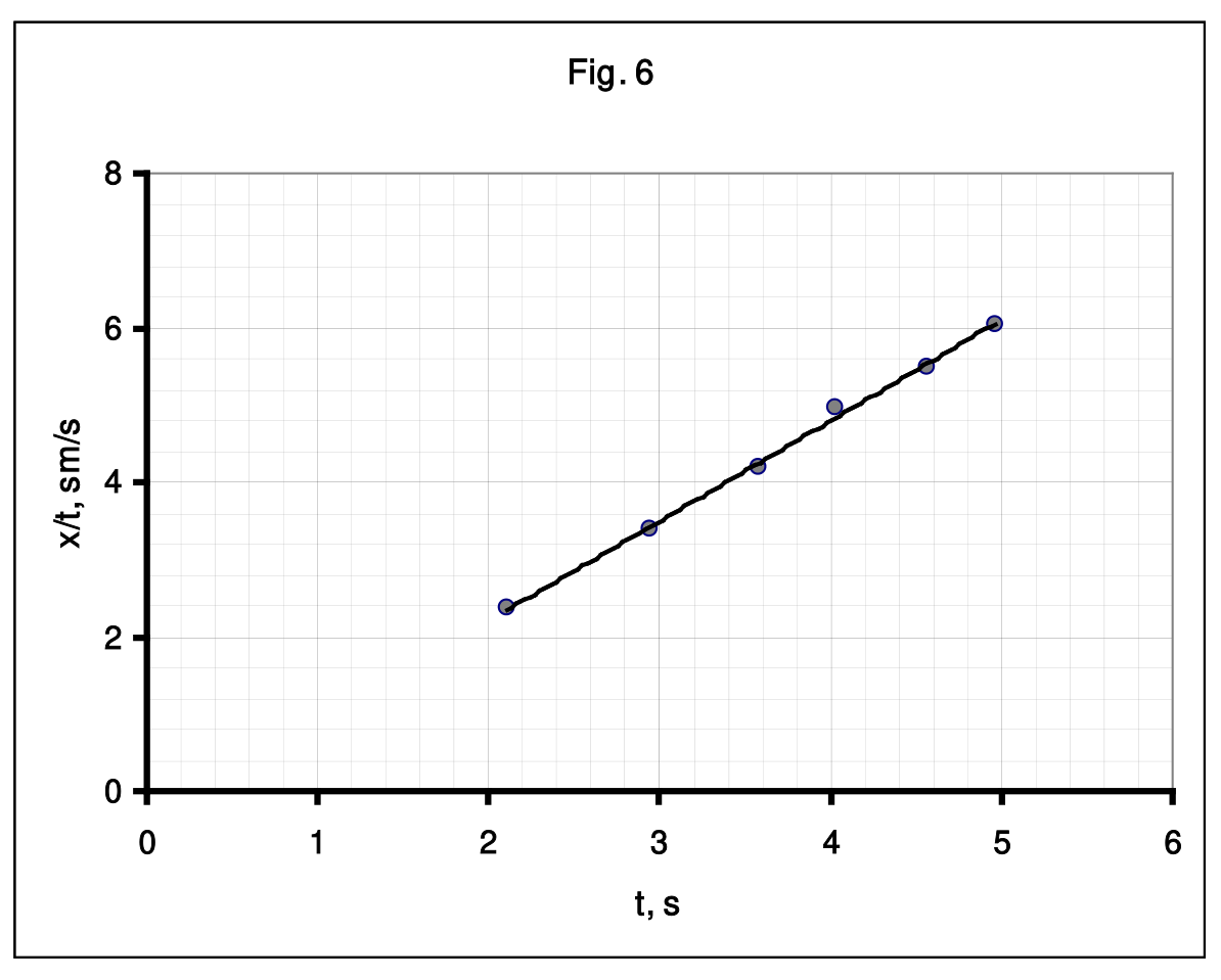
To calculate the acceleration, we use the previous methodology: we draw the dependence $\frac{x}{t}$ on $t$ (Fig. 6) and find the parameters of the linearized dependence.

The least squares calculations give the following values of the coefficients of the dependence $\frac{x}{t} = Kt + b$ :

K = (1{,}30 \pm 0{,}07)\frac{sm}{s^2}

b = (-0{,}40 \pm 0{,}3)\frac{sm}{s}

Fig. 5: graph of x, sm (0 to 35) versus t, s (0 to 5) with the data of Table 4 on a parabola-like curve starting at the origin.

Fig. 6: graph of x/t, sm/s (0 to 8) versus t, s (0 to 6) with six points from t ≈ 2,1 s to 5,0 s lying on a straight line from about 2,4 to 6,1.

Then, the disc axis acceleration is found as

a = (2{,}60 \pm 0{,}13)\frac{sm}{s^2}. \qquad (7)

2.3 The formula for the acceleration is automatically obtained from formula (2), in which $\sin\alpha = 1$ :

a = \frac{g}{1+\frac{1}{2}\left(\frac{r}{R}\right)^2}. \qquad (8)

The calculation using this formula gives the value of $a = 2{,}44\frac{sm}{s^2}$ .

Part 3. Moving up

3.1 Threads should be wound such that when the threads tied to the load are untwisted, the threads attached to the Maxwell disk are twisted. It is also obvious that the threads with the load should be wound on a part of the stick with a larger radius.

Side view of the disc (large circle) and the stick (small circles at the centre) showing the winding of the threads: one thread leaves the stick going up, another going down, with curved arrows showing the direction of winding.

3.2 In this case, the beginning of the motion of the disk axis is easily recorded, so you can simply measure the rise time to a fixed height and calculate the acceleration according to the formula:

H = \frac{at^2}{2} \quad\Rightarrow\quad a = \frac{2H}{t^2}. \qquad (9)

During the measurements, the following data shown in Table 5 (at $H = 12sm$ ) have been obtained.

Table 5

$n$	$t_1$ , s	$t_2$ , s	$t_3$ , s	$\langle t \rangle$ , s	$a$ $\frac{sm}{s^2}$
1	2,07	2,13	2,23	2,14	5,22
2	1,6	1,56	1,63	1,60	9,41

Marking scheme

	Content	Total points for parts	Points
Part 1. Rolling down		8
1.1	Formula (2) $a = \frac{g}{1+\frac{1}{2}\left(\frac{r}{R}\right)^2}\sin\alpha$	0,3	0.3
1.2	Experimental setup is properly designed; appropriate data are obtained by order of magnitude	0,5	0,5
	The value of $\sin\alpha$ is stated: Measurement method; Numerical value lies in the range of 0,04 – 0,2;	0,2	0,1 0,1
	The dependence measurement Marked only if $\sin\alpha$ is in the range above, Data deviation from the official solution is within 25%: - range of coordinate measurement exceeds 20 sm (exceeds 10 sm, less than 10 sm); - number of data points 5 and more (4, less than 4); - the nonlinear dependence is obtained which is close to parabolic;	1,2	0,5(0,3;0) 0,5(0,3;0) 0,2
	Graph of $x(t)$ (marked only if the corresponding data have been marked): - axes are named and ticked; - all data points are in the graph; - smooth curve is plotted;	0,3	0,1 0,1 0.1
	Analysis of the uniform acceleration model: - the law of motion $x(t) = v_0 t + \frac{at^2}{2}$ ; - Without the initial velocity;	0,2	0.2 (0)
	The analysis methodology: - linearization $\frac{x}{t} = v_0 + \frac{a}{2}t$ ; - calculation of velocities $v(t)$ ; - linearization $x(t^2)$ ; - acceleration calculation by 2-3 points;	1,0	1 (0,5) (0.2) (0.1)
	Graph of the linearized dependence (marked only if corresponding data have been marked): - axes are named and ticked; - all data points are in the graph; - smooth curve is plotted;	0.3	0,1 0,1 0.1
	Calculation of the acceleration (not marked if there is no unit); - according to the linearized dependence (LSM, graph); - by 2-3 points; - by 1 point;	0,4	0,4 (0,2) (0,1)
1.3	Acceleration dependence on the angle Marked only if data deviation from the official solution is within 25%: Sine of the angle is within the range 0,04 – 0,2 : - number of angles taken is 4 or more (3, less than 3); - number of data points in each dependence is 5 or more (3-4; less than 3);	1,4	0,2 0,8 (0,5;0) 0,4(0,2;0)
	Acceleration calculation (for each point but no more than 4): - linearization; - by 1-3 points; Calculation of $\sin\alpha$ ;	1,0	0,2х4 (0,1х4) 0.2
	Graph of the angle dependence of the acceleration (marked only if corresponding data points have been marked): - axes are named and ticked; - all data points are in the graph; - smooth curve is plotted;	0,3	0.1 0,1 0.1
1.4	Disc and stick radii are measured; Correct formula is used for calculations; Linear dependence is drawn; Experimental data lie systematically below the theoretical curve;	0,9	0,2 0,1 0,1 0,5
Part 2. Moving down		4
	Experimental setup is properly designed; appropriate data are obtained by order of magnitude	0,5	0,5
2.1	Experimental data Marked only if data deviation from the official solution is within 25%: - the range of the coordinate measurements exceeds 20 sm (exceeds 10 sm; less than 10); - number of data points is 5 or more (3-4; less than 3); - average is done by 3 or more repetitions; - the dependence close to parabolic is obtained;	1,5	0,5(0,3;0) 0,5(0,3;0) 0,3 0,2
	Graph of $x(t)$ (marked only if corresponding data have been marked): - axes are named and ticked; - all data points are in the graph; - smooth curve is plotted;	0,3	0,1 0,1 0.1
2.2	Acceleration calculations (marked only if corresponding data have been marked): - linearization is used (allowed to use $x(t^2)$ ; - acceleration is calculated using the linearized dependence (by 1-2 points); - experimental error is calculated;	1,3	0,5 0,5 0,3
2.3	Correct formula for the acceleration is derived; Numerical value is correctly evaluated;	0.4	0,2 0.2
Part 3. Moving up		3
3.1	Correct schematic figure for wounding the threads (threads are on one side of the stick);		1
3.2	Time of moving up is measured (within the range of 0,7 – 3,0 s)		0,5х2
	Accelerations are calculated (within 50% deviation from the official solution)		0,5х2
	Total	15

Оригинал в Архива: IZhO-2020-Exp_eng.pdf · официални решения: IZhO-2020-Exp_eng_sol.pdf