IZhO 2022 — Задача 2. Experiment 2: Rolling friction

XVIII International Zhautykov Olimpiad/Experimental Competition · 17 февруари 2022 г.

Условие

Please read this first:

1. The duration of the experimental competition is 4 hours. There are two problems.

2. You can use your own calculator for numerical calculations.

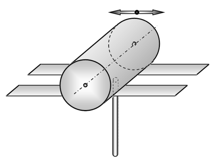
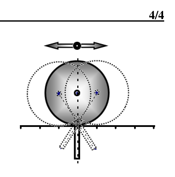
In reality, even in the absence of slipping between the bodies, there are frictional forces called rolling friction forces. In this experiment, the following setup is used to study the rolling friction. A small rod is rigidly attached to the side surface of a massive solid cylinder, whose imaginary prolongation crosses the axis of the cylinder. The cylinder is located on the two horizontal plates so that it can roll over them without slipping. In this case, the rod lies always in the gap between the plates.

Let us use the following notation: the radius of the cylinder $R$, the mass of the cylinder $M$, the mass of the attached rod $m$, which can be considered significantly less than the mass of the cylinder, the distance from the center of mass of the rod to the axis of the cylinder $l$.

Usually, the formula for the rolling friction force is written as

$F = \frac{\kappa}{R}N\,,$

where $N$ is the normal reaction force, $R$ stands for the radius of the rolling body, and $\kappa$ refers to the rolling friction coefficient. In this part of the problem, it is necessary to determine the dimensionless value $\mu_r = \dfrac{\kappa}{R}$, which for brevity is called the coefficient of rolling friction. Typically, the coefficient of rolling friction is much less in magnitude than the coefficient of sliding friction studied above.

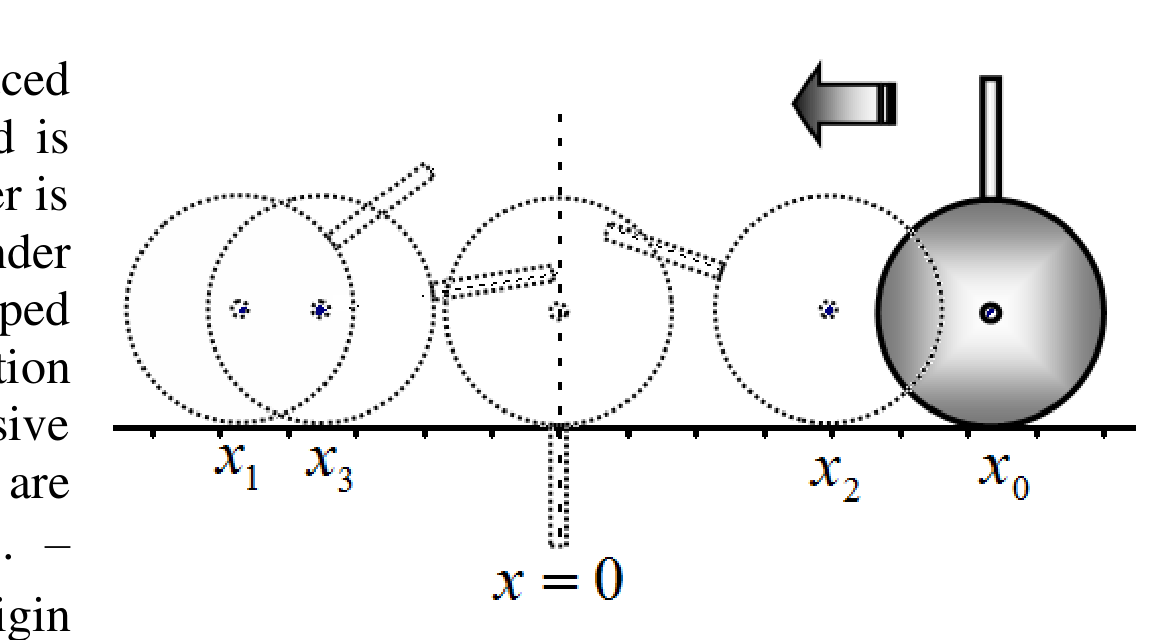
During the experiment, the cylinder is placed into its initial position in such a way that the rod is directed vertically upwards, after which the cylinder is released without any significant push. The cylinder starts to roll on the plates, performing damped oscillations due to the action of the rolling friction force. In this case, the coordinates of successive extreme positions of the cylinder (stoppage points) are written down: $x_0$ – initial position, $x_1, x_2, x_3\dots$ – coordinates of successive stoppage points. The origin of coordinates $x=0$ corresponds to the point where the rod is directed vertically downwards. Table 2 shows the experimental values of the coordinates of the stoppage points, whose measurement error is found as $\Delta x = 0{,}2\,sm$.

Table 2. Coordinates of the stoppage points.

$k$	$x_k$, sm
0	15,8
1	-11,6
2	10,1
3	-9,0
4	7,7
5	-7,0
6	5,7
7	-5,3
8	4,7
9	-3,9
10	2,8

To determine the setup parameters, the period of small oscillations of the cylinder near the equilibrium position (point $x=0$) is measured. For this, the times of five oscillations of the cylinder with the rod are measured several times. The results of these measurements are shown in Table 3. The instrumental error of the time measurement is $\Delta t = 0{,}02s$

Table 3. The times of five oscillations

$k$	$t_5$, s
1	7,39
2	7,21
3	7,26
4	7,47
5	7,44

2.1 Derive the formula for the period of the small fluctuations described right above. Express the oscillation period in terms of the setup parameters $M, m, R, l$ and the free fall acceleration $g$.

2.2 Derive an equation relating the coordinates of two successive cylinder stoppage points $x_k, x_{k-1}$ in the described cylinder rolling experiment. This equation, in addition to the coordinates, may include the setup parameters $M, m, R, l$, the free fall acceleration $g$ and the coefficient of rolling friction $\mu_r$.

2.3 Express the coordinate of the $k$'th cylinder stoppage point in terms of the initial coordinate $x_0$ and the coordinates of all previous stoppage points $x_1, x_2, \dots x_{k-1}$. This equation, in addition to the coordinates of the stoppage points, should include only the free fall acceleration g and the period of small oscillations $T$.

2.4 Using the measurement results given in Table 3, calculate the period $T$ of small oscillations of the cylinder. Estimate the measurement error $\Delta T$ of this quantity.

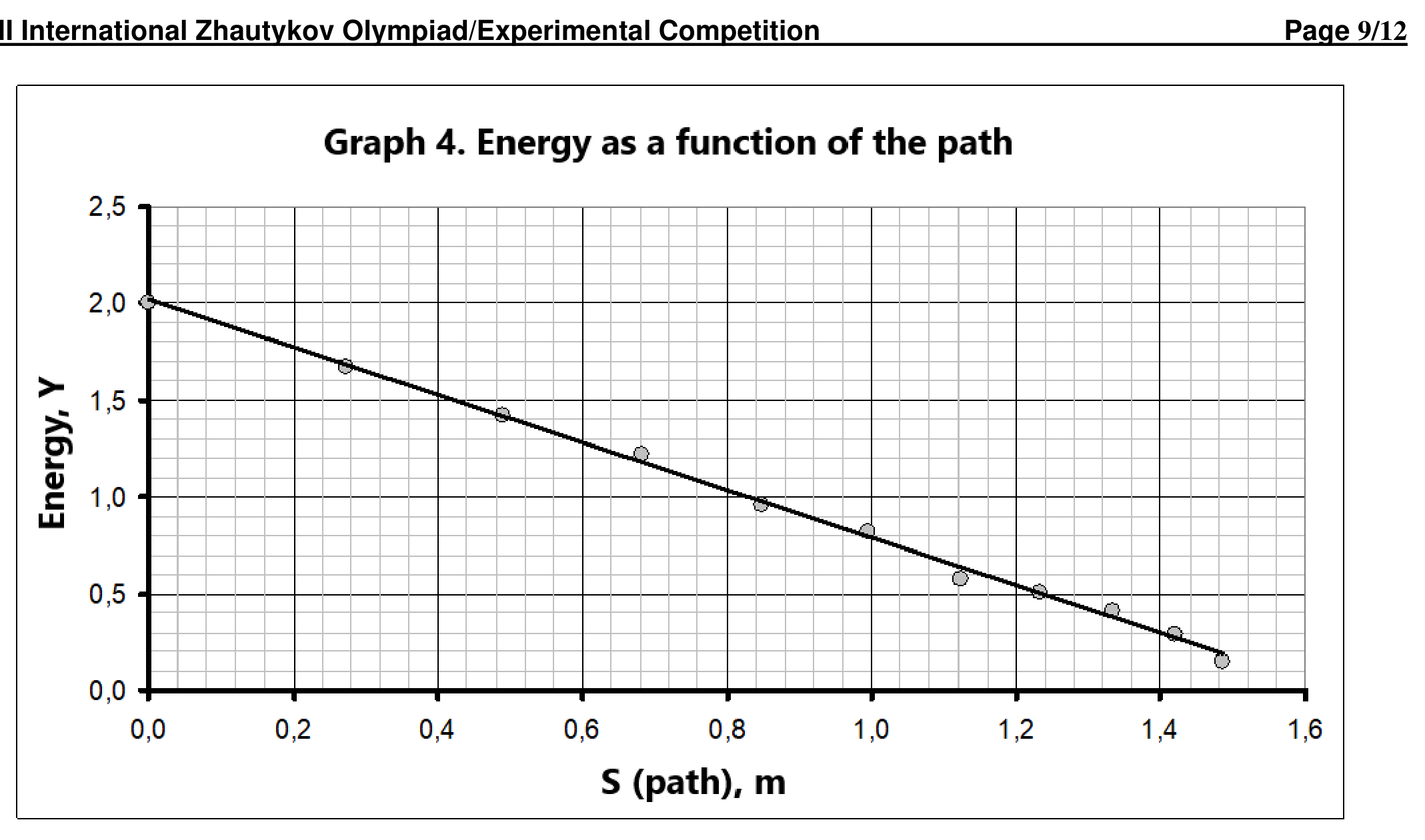
2.5 Propose such values $Y(x_k)$ and $X(x_0, x_1, \dots x_k)$ such that the dependence $Y(X)$ turns linear and allows you to calculate the coefficient of rolling friction $\mu_r$. Draw a graph of the linearized relationship $Y(X)$.

2.6 Using the linearized relationship $Y(X)$, calculate the coefficient of rolling friction $\mu_r$. Estimate the error $\Delta\mu_r$ of the obtained value.

Решение

---

Оригинал в Архива: IZhO-2022-Exp_eng.pdf · официални решения: IZhO-2022-Exp_eng_sol.pdf