NBPhO 2025, Теория и експеримент — Задача 9. Hot Plate

i) (3 т.)

Both aluminium plates were immersed in hot water until thermal equilibrium was reached, then removed, dried with tissue paper, and measured using an infrared thermometer. The plates have identical thermal properties except for their surface coating, so they should have reached the same actual temperature in the hot water bath. Experimental measurements:

The infrared thermometer measures temperature based on thermal radiation and we were told it is calibrated for emissivity $\varepsilon = 1$ (in reality, it is calibrated for $\varepsilon = 0.95$, but this difference is not significant). We were also told that the radiation power can be linearized: $P_{\mathrm{thermal}} = P_0 + \alpha T$. Objects with $\varepsilon < 1$ radiate $P_\varepsilon = \varepsilon(P_0 + \alpha T_\varepsilon)$, but they also reflect/scatter the radiation falling onto it from the environment. If the room is more or less at the thermal equilibrium at temperature $T_0$, the room is filled with the photons at thermal equilibrium with walls at temperature $T_0$. If the plate were to be black and also at temperature $T_0$, it would be in equilibrium with the radiation and emit $P = P_0 + \alpha T_\varepsilon$; so, there must be as much incident radiation from the surroundings regardless of its real emissivity and temperature. As it follows from the second law of thermodynamics, the reflectance must be $1 - \varepsilon$, so it reflects/scatters power equal to $P_r = (1 - \varepsilon)(P_0 + \alpha T_0)$. This means that the total power departing from it is $P_\varepsilon + P_r = P_0 + \varepsilon\alpha T_\varepsilon + (1 - \varepsilon)T_0$. The IR thermometer assumes this is a black body and equates this power to $P_0 + \alpha T_{\mathrm{reading}}$, hence were density as would have a room thermometer reading is a weighted average:

Since the black plate has $\varepsilon = 1$, its reading directly gives the actual temperature of both plates. Rearranging to solve for emissivity:

Calculating for each measurement:

Taking the average: $\varepsilon = \frac{0.069+0.065+0.053}{3} = 0.062 \approx 0.06$ The emissivity of the polished aluminium plate is $\varepsilon = 0.06 \pm 0.01$.

Grading: (preliminary)

• The idea of heating the two plates together in water (using alternative methods doesn’t guarantee equal temperatures for the plates well) 0.4 pts
• Measuring the radiance of the plates in a properly (plates are properly dried and measurements are done in a timely manner) 0.4 pts
• Making at least three measurements of the black plate, the polished plate and the surrounding environment (0.2 p for each set of 3, totalling) 0.6 pts
• Understanding that the IR temperature reading of the polished plate is affected not only by the plate itself, but also by the reflected radiation of the environment $T_{\mathrm{reading}} = \varepsilon\cdot T_{\mathrm{actual}} + (1 - \varepsilon)\cdot T_{\mathrm{ambient}}$ , not just $T_{\mathrm{reading}} = \varepsilon\cdot T_{\mathrm{actual}}$ 0.3 pts
• Deriving a correct formula for emissivity, expressed in terms of the three measured temperatures 0.7 pts
• Calculated value of emissivity in the range from 0.03 to 0.12 0.6 pts (for values from 0.02 to 0.2: 0.4 pts, for values from 0.01 to 0.3: 0.2 pts).

ii) (3 т.)

Solution 1. Here the main idea is to heat the plate using the resistor. Once thermal equilibrium is reached with plate’s temperature $T = T_f$, the heating power $P = V^2/R$ equals to the power dissipated to the environment, $H(T_f - T_0)$ (with $T_0$ denoting the room temperature), hence we can determine the heat exchange coefficient as $H = V^2/R(T_f - T_0)$. The main difficulty with this approach is that the characteristic thermalization time is long, around 7 minutes, so for a more or less precise measurement, one should wait around half an hour.

Grading: (preliminary)

• The idea of using resistive heating and waiting for thermalization 0.5 pts
• For waiting long enough, up to 0.8 pts ;as follows: for each five minutes missing from more than 30 minutes, subtract 0.2 pts (so, less than 30 minutes is 0.8 pts; less than 25 minutes is 0.6 pts ... etc).
• The voltage is maximized to have maximal $T_f$ (needed to reduce the relative error of $T_f - T_0$ 0.4 pts (the maximal allowed voltage of $15\ \mathrm{V}$ gives maximal points, each missing volt subtracts 0.1 pts.
• Measuring the temperature and obtaining a value that is reasonable for the given voltage, i.e. difference is not bigger than $1\ ^{\circ}\mathrm{C}$ 0.6 pts
• Deriving a correct formula for $H$ 0.5 pts
• Evaluating correctly 0.2 pts (any mistake, either with units or arithmetic, leads to no points)

Solution 2. In order to avoid long waiting time, the following approach can be used. Although it involves more complicated data analysis, the analysis results are re-usable by part iii.

The black aluminium plate was placed on the foam plastic with the resistor beneath it, providing continuous heating. Temperature readings were recorded at one-minute intervals (the first row shows time in minutes, the second — the measured temperature in °C:

For heating with constant power, the temperature evolution follows $T = T_f - \theta\mathrm{e}^{-\gamma t}$, where $T_f$ is the final equilibrium temperature, $\theta$ is a constant depending on the initial temperature, and $\gamma$ is the inverse of the characteristic time constant. To determine $\gamma$, we examine successive temperature increments $T(t + \tau) - T(t) = \theta\mathrm{e}^{-\gamma t}(\mathrm{e}^{\gamma\tau} - 1)$ with $\tau = 1\ \mathrm{min}$, which should decrease exponentially, i.e. $\ln\Delta T \equiv \ln[T(t + \tau) - T(t)] = -\gamma t + \mathrm{const}$ should be a linear function of time.

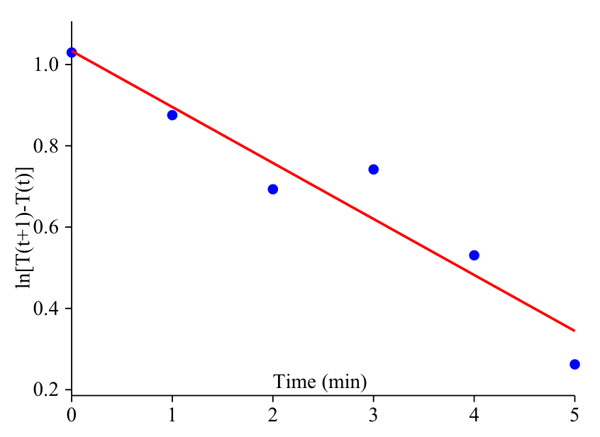
Linear regression analysis of $\ln[T(t + 1) - T(t)]$ versus $t$ yields:

with $R^2 = 0.9209$ indicating a good fit. Thus we obtain $\gamma = 0.1378\ \mathrm{min^{-1}}$, corresponding to the time constant of the thermal system $1/\gamma \approx 7.3$ minutes.

We now plot $T$ versus $\mathrm{e}^{-\gamma t}$ to find $T_f$ as the intercept when $\mathrm{e}^{-\gamma t} = 0$:

Computing $\mathrm{e}^{-0.1378n\tau}$, $n = 0, \dots 6$ values yields

the corresponding plot is provided below.

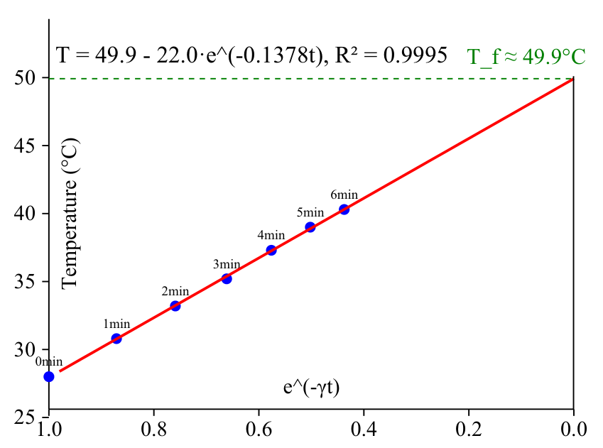
Linear regression of $T$ versus $\mathrm{e}^{-\gamma t}$ yields $T_f \approx 49.9^{\circ}C$, as shown in the equation:

with $R^2 = 0.9995$ indicating an excellent fit. At thermal equilibrium, the power dissipated equals the power supplied:

where $h$ is the heat transfer coefficient per unit area, $H$ is the total heat transfer coefficient, $A$ is the plate area, $U$ is the applied voltage, and $R$ is the resistor’s resistance. Using $U = 15\ \mathrm{V}$, $R = 220\ \Omega$, $A = 40\times 40\ \mathrm{mm^2} = 1.6\times 10^{-3}\ \mathrm{m^2}$, and $T_0 = 22.9\ ^{\circ}\mathrm{C}$ we obtain

The total heat transfer coefficient $H$ is found as

Grading: (preliminary)

• Coming up with the idea of analysing exponential decay of temperature change with a graph and deriving the heat transfer coefficient from that 0.5 pts
• Correct equation $T(t) = T_f - \theta\mathrm{e}^{-\gamma t}$. 0.3 pts
• Plotting the data to a graph to determine the $\gamma$ and to confirm the validity of collected data 0.3 pts
• At least 5 datapoints used. 0.1 pts
• Measure for at least 5 minutes. 0.1 pts
• Calculating the slope and retrieving $\gamma$ from it. 0.2 pts
• Finding the maximal temperature for used voltage used, using plot of $T$ vs $e^{-\gamma t}$. 0.5 pts
• Evaluating $P = \frac{U^2}{R} = h\cdot A\cdot(T_f - T_0) = H\cdot(T_f - T_0)$ without errors 0.5 pts
• Getting heat Transfer coefficient close to expected value 0.5 pts

iii) (2 т.)

Solution 1 To determine the heat capacity, we can use the heating curve from Part 2. During heating, the energy balance is written as

where $P_{\mathrm{in}} = U^2/R$ is the input power, $P_{\mathrm{out}} = H(T - T_0)$ (where $T_0 = T_{\mathrm{room}}$ is the room temperature) is the power lost to the environment, $C$ is the heat capacity, and $\frac{\mathrm{d}T}{\mathrm{d}t}$ is the rate of temperature change. Using our exponential model $T = T_f - \theta\mathrm{e}^{-\gamma t}$, we find:

Substituting into the energy balance:

This allows us to calculate the heat capacity $C$ as

Now we need to use the values from Parts 1 and 2:

The input power is evaluated as

For each time point, we can calculate:

The heat capacity values are remarkably consistent across different time points, which validates our model. Taking the average of the values in the tableˊyields

This value represents the heat capacity of the aluminium plate. For reference, the specific heat capacity of aluminium is approximately $c_{\mathrm{Al}} = 900\ \mathrm{J\,kg^{-1}\,K^{-1}}$, which means the plate has a mass of about $C/c_{\mathrm{Al}} = 18.3\ \mathrm{g}$. This is a reasonable value for a $40\ \mathrm{mm}\times 40\ \mathrm{mm}$ aluminium plate with a thickness of approximately $2\ \mathrm{mm}$.

Solution 2. The calculated heat capacity represents the effective heat capacity of the system as observed in the experiment. This includes the aluminium plate and potentially some contribution from the heating resistor and its mounting. Therefore, a little better approach is to make an additional series of measurements to obtain a cooling temperature curve (similar to those what will be made in the next section), because then we could have let the plate cool on a flat part of the foam plastic, excluding thereby the contribution of the resistor’s thermal capacity. If part ii was solved using the solution 1, this is the only viable way.

So, we heat the plate — the easier way is by immersing into hot water — and measure the time and temperature as it cools down. As a result, we obtain data about $T(t)$; the energy balance equation is

hence

Similarly to the solution 1, we have used the fact that the plate cools exponentially in time and hence, $\frac{\mathrm{d}T}{\mathrm{d}t} = \gamma[T(t) - T_0]$. The decay rate can be found by plotting $\ln[T(t) - T_0]$ against $t$ and determining the slope of the linear fit line.

• The idea of using the $T(t)$ dependence, either for cooling or heating with the resistor 0.2 pts
• Measuring and tabulating at least 6 data points 0.3 pts (subtract 0.1 pts for each missing)
• Data points cover at least 6 minutes 0.3 pts (subtract 0.1 pts for each missing minute)
• The idea of using log-linear plot for data linearization 0.2 pts
• Correct data plotting 0.2 pts
• Finding the slope of a fit line 0.2 pts
• The idea of substituting time derivative with multiplication by $\gamma$ 0.2 pts (alternative approach of calculating derivative by finite difference ratio $\Delta T/\delta t$ is significantly less accurate).
• Deriving a correct formula for $C$ 0.2 pts
• Obtaining a reasonable numerical value for $C$, i.e. from $13\ \mathrm{J\,K^{-1}}$ to 20 — 0.2 pts (else from 10 to 25: 0.1 pts).

iv) (4 т.)

For this part, cooling experiments were conducted with the aluminium plate covered by different numbers of silicone rubber layers. The plate was heated in water and then allowed to cool, with temperature recorded as a function of time.

*The data point at $t = 0$ for 2 layers is excluded as it did not represent complete thermal equilibrium across the silicone layers. For a cooling process with constant ambient temperature, the temperature follows an exponential decay:

The time constant $\gamma$ is related to the thermal resistance $\mathcal{R}$ and heat capacity $C$ by

Taking the natural logarithm of the temperature difference from ambient yields

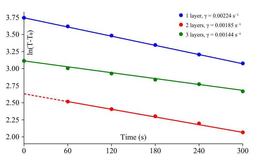
Using linear regression on the logarithmic cooling curves, we obtain:

Using our previously determined heat capacity $C = 16.5$ J/K, we calculate the total thermal resistance for each case:

The total thermal resistance includes the resistance of the silicone layers and the thermal resistance of convection and radiation. Each additional layer adds a resistance $\Delta R = \delta/(\kappa A)$, where $\delta$ is the layer thickness, $\kappa$ is the thermal conductivity, and $A$ is the area. The incremental resistances between layers are:

Taking the average incremental resistance per layer:

With the silicone rubber pad thickness $\delta = 0.8$ mm $= 8\times 10^{-4}$ m and area $A = 40\times 40$ mm$^2 = 1.6\times 10^{-3}$ m$^2$, we can calculate the thermal conductivity:

The precision of this experiment can be increased by longer runs and adding additional silicon layers.

• The idea of letting the plate to cool down while covering it with a different number of silicon sheets and measuring the $T(t)$ dependencies, 0.3 pts
• For the quantity of recorded data: within each data series (i.e. a series with a different number of silicon sheets), at least 6 data points: 0.3 pts (subtract 0.1 for each missing), within up to three different data series — in total up to $3\times 0.3$pts, i.e. 0.9 pts
• Data points in each data series cover at least 6 minutes: 0.2 pts (0.1 pts if less than 6 but more than 4 minutes) — in total up to 0.6 pts
• The idea of using log-linear plot for data linearization 0.2 pts
• Correctly plotting the data: 0.1 pts each, up to 0.3 pts
• Calculating $\gamma$ for each of the series, 0.1 pts for each (up to for three data series), in total up to 0.3 pts
• Correctly expressing the heat conductivity in terms of a difference of the $\gamma$ values 0.7 pts
• Finding conductivity on the basis of all the $\gamma$ values (either by pair-wise calculation, or plotting and finding the fit line slope 0.4 pts (divide by two if only one pair of $\gamma$ values was used)
• Obtained value of $\kappa$ within a reasonable range, i.e from 0.05 to $0.1\ \mathrm{W\,m^{-1}\,K^{-1}}$: 0.3 pts (else if from 0.04 to 0.12: 0.2 pts; else from 0.02 to 0.14: 0.1 pts).