OPhO 2022, Теория — Задача 5. Quantum Computing
2022 Online Physics Olympiad: Invitational Contest — Theoretical Examination · 26 т.
Sponsors
This competition could not be possible without the help of our sponsors, who are all doing great things in physics, math, and education.
The original sponsor marks link to Jane Street, Wolfram, AwesomeMath, Beyond the Big Bang, Physics Olympiad, and AoPS Art of Problem Solving.
Instructions for Theoretical Exam
The theoretical examination consists of 5 long answer questions and 110 points over 2 full days from July 30, 0:01 am GMT.
- The team leader should submit their final solution document in this google form. We don’t anticipate a tie, but in the rare circumstance that there is one, the time you submit will be used to break it.
- If you wish to request a clarification, please use this form. To see all clarifications, view this document.
- Participants are given a google form where they are allowed to submit up-to 1 gigabyte of data for their solutions. It is recommended that participants write their solutions in LaTeX. However, handwritten solutions (or a combination of both) are accepted too. If participants have more than one photo of a handwritten solution (jpg, png, etc), it is required to organize them in the correct order in a pdf before submitting. If you wish a premade LaTeX template, we have made one for you here.
- Since each question is a long answer response, participants will be judged on the quality of your work. To receive full points, participants need to show their work, including deriving equations. As a general rule of thumb, any common equations (such as the ones in the IPhO formula sheet) can be cited without proof.
- Remember to state any approximations made and which system of equations were solved after every step. Explicitly showing every step of algebra is not necessary. Participants may leave all final answers in symbolic form (in terms of variables) unless otherwise specified. Be sure to state all assumptions.
Problems
- T1: Maxwell’s Demon
- T2: Euler’s Disk
- T3: Rocket
- T4: Magical Box
- T5: Quantum Computing
List of Constants
- Proton mass,
- Neutron mass,
- Electron mass,
- Avogadro’s constant,
- Universal gas constant,
- Boltzmann’s constant,
- Electron charge magnitude,
- 1 electron volt,
- Speed of light,
- Universal Gravitational constant,
- Acceleration due to gravity,
- 1 unified atomic mass unit,
- Planck’s constant,
- Permittivity of free space,
- Coulomb’s law constant,
- Permeability of free space,
- Stefan-Boltzmann constant,
Problem writers
T1: Maxwell’s Demon — Zhening Li
T2: Euler’s Disk — Daniel Seungmin Lee
T3: Rocket — Adithya Balachandran
T4: Magical Box — Daniel Seungmin Lee
T5: Quantum Computing — QiLin Xue
Organizer clarification document — major notes
Separately quoted from the organizer clarification document, titled 2022 OPhO Invitational Theory Clarifications:
MAJOR NOTES
- Last updated: July 30, 12:01 am UTC
- We will only be adding clarifications that cannot already be found in the exam. If you are not seeing your clarification answered, try looking through the exam again to see if you did not miss anything.
The separate Experimental Notes link is retained in the original clarification PDF and concerns the distinct experimental paper.
Условие
In this problem, you will learn the fundamentals of quantum computers, as well as the physics on how they can be constructed! We have tried to provide as much background information as necessary, but if you believe some part is missing or unclear, please fill out the clarifications form.
Introduction
Physicists use braket notation to describe vectors in quantum systems. When using a vector to describe a quantum state, the ket, written as can be used. Both notations below are equivalent:
The bra, on the other hand, is the conjugate transpose of the ket . Given two vectors and , the braket is the inner product of both vectors. This notation will be used throughout this problem.
In any digital device, information is communicated via 0s and 1s, or binary code. The simplest units of this information are called bits. Similar to a bit, the qubit can be represented as a linear combination of two orthogonal states: quantum-0 and quantum-1, which are typically and . Here,
Typically, we write a single qubit state as
where , and .
a. (1 pt.) A qubit is prepared in the state .
(i) What is the probability of measuring the qubit in the state ?
(ii) What is the probability of measuring the qubit in the state ?
Hint: If you are still confused about measurement (it’s tricky!), check out this qiskit article. You can ignore all the parts with code, we’ll save those for the computer science students writing OCSO.
A quantum gate performs an unitary operator on a quantum state. Applying an operator (sometimes known as a gate) to a qubit state can be represented in the diagram below.

where is a local unitary since it only acts on a single qubit. There are five important gates:
Here, form the four Pauli matrices and is known as the Hadamard gate, which we will use later on when we talk about entanglement.
For example, if and apply the gate , we end up with
b. (1 pt.) A qubit is prepared in the state . What is the probability of measuring the qubit in the state ? Express your answer in terms of , and properties of the unitary .
The heart of quantum information lies in what we can do with more than a single qubit. If one qubit has two dimensions ( and ), then a two-qubit system can be represented in four dimensions. For a two qubit system, the state can be written as , where can be seen as the “basis vectors.” If we have two independent qubits, i.e. and , we can represent their combined state using the tensor product, i.e.
Here, we can see that
Note that not every two qubit state can be written as a tensor product. When this occurs, we say that they are entangled. We can immediately determine if a state is entangled by calculating its concurrence, defined by
If , then the two qubits are separate and the system is separable. If , the system is maximally entangled, such as
Physically, this means that a measurement of one qubit directly leads to a “collapse” of the other qubit (this is the classic example shown in popular science media). Note that .
We can change the concurrence using a control operation. For example,
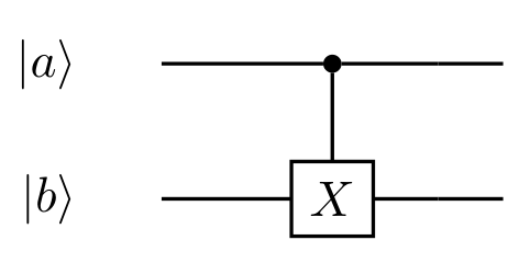
performs the CNOT gate. The unitary is applied to if , otherwise nothing is done. That is, we have:
The CNOT gate is an example of a global unitary, since it acts on more than one qubit. Global unitaries for 2 qubit systems can be written as a matrix. For example, we can write
where form the 4 standard basis vectors. We can combine local and global unitaries to create entangled states. For example, consider the following circuit:
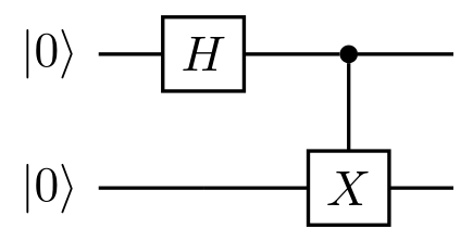
The initial state is . After applying the Hadamard gate , the state becomes
After applying the CNOT gate, the state becomes:
Note that we can avoid matrix multiplication in this last step by seeing what CNOT does on each term of . CNOT will not have an effect on since the first qubit is . CNOT will have an effect on since the first qubit is a , so it’ll flip the second qubit to a , giving us the map .
c. (1 pt.) Construct a quantum circuit where the input state is and the output state is using only gates.
Quantum Teleportation
Quantum teleportation is the transfer of the quantum state of one qubit to another (not the actual physical qubit) using a shared entangled resource and two classical bits of information. It is performed using the following circuit.
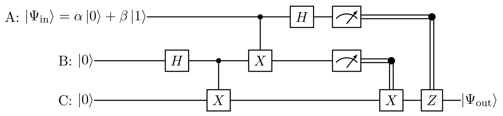
The gate measures the qubit (returns either a 0 or a 1) and the wider wire represents that information that flows through this wire is a classical bit.
d. (1 pt.) Verify that the above circuit does teleport the qubit from the top branch to the bottom branch by looking at the specific case of
e. (3 pts.) After the first operation is performed on branch , the branch is brought a very far distance from the other two branches. By doing so, it appears we can create faster-than-light communication during the teleportation process, which is impossible! Explain why there is no contradiction. Justify rigorously.
We can analyze this by performing matrix multiplication, but using a circuit-based approach is much cleaner. To do so, we need to use the Griffiths-Niu Theorem.
f. (2 pts.) The following circuits, according to the Griffiths-Niu Theorem, are equivalent:
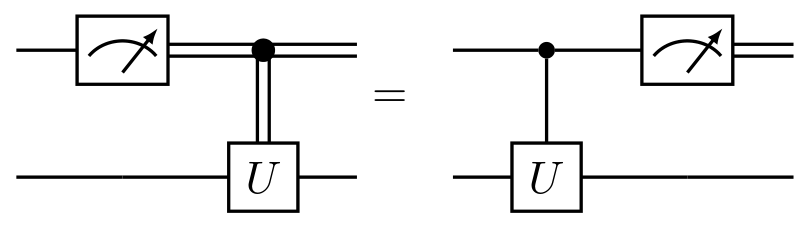
Prove the Griffiths-Niu Theorem.
Using this theorem, we can redraw our circuit as:
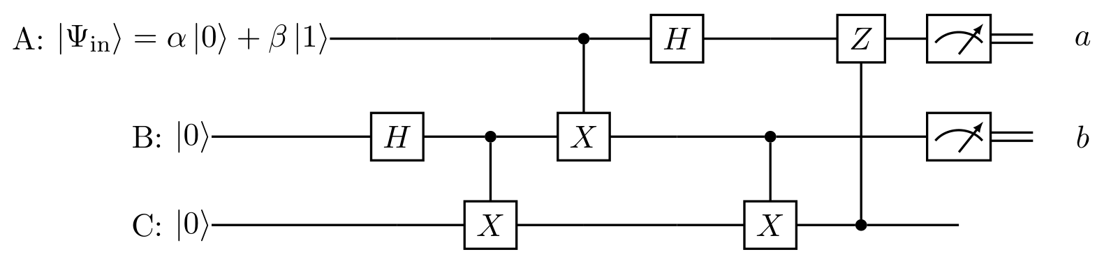
g. (1 pts.) For a control-Z gate, it doesn’t matter which branch is the control. In other words,
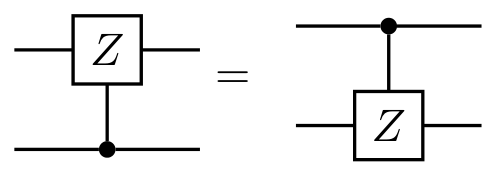
Prove this relationship.
Using the above problem, we can flip the control-Z gate. Then using the identity , we can reduce it further:

Since , we can simplify the top part. Furthermore, we can introduce another CNOT between the first and the second branch.
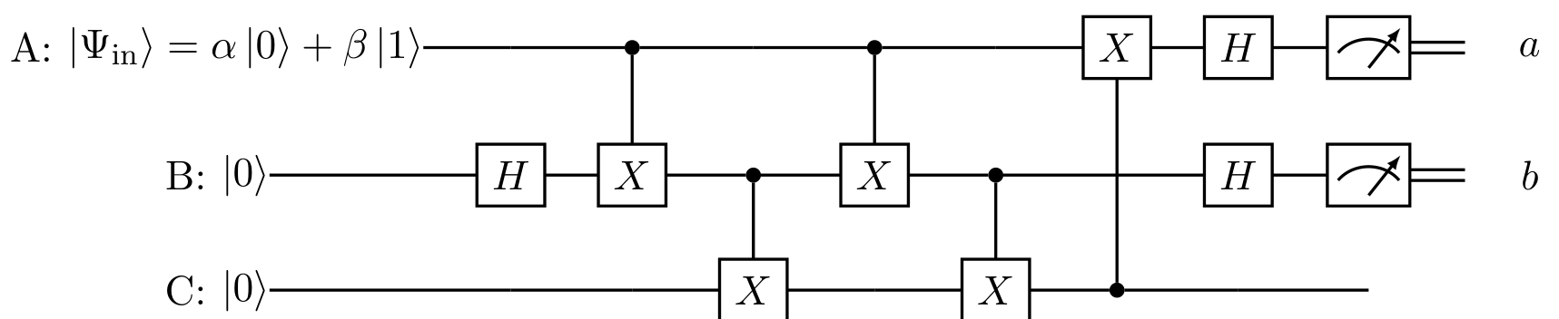
We were allowed to introduce this CNOT gate since . This actually makes it easier using the following problem:
h. (2 pts.) Prove that the below two circuits are equivalent.
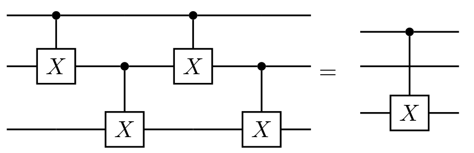
Using this substitution, we end up with:
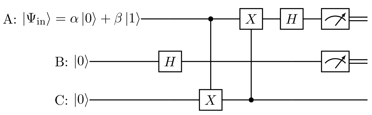
We can now introduce another CNOT gate, which doesn’t do anything since will always be .
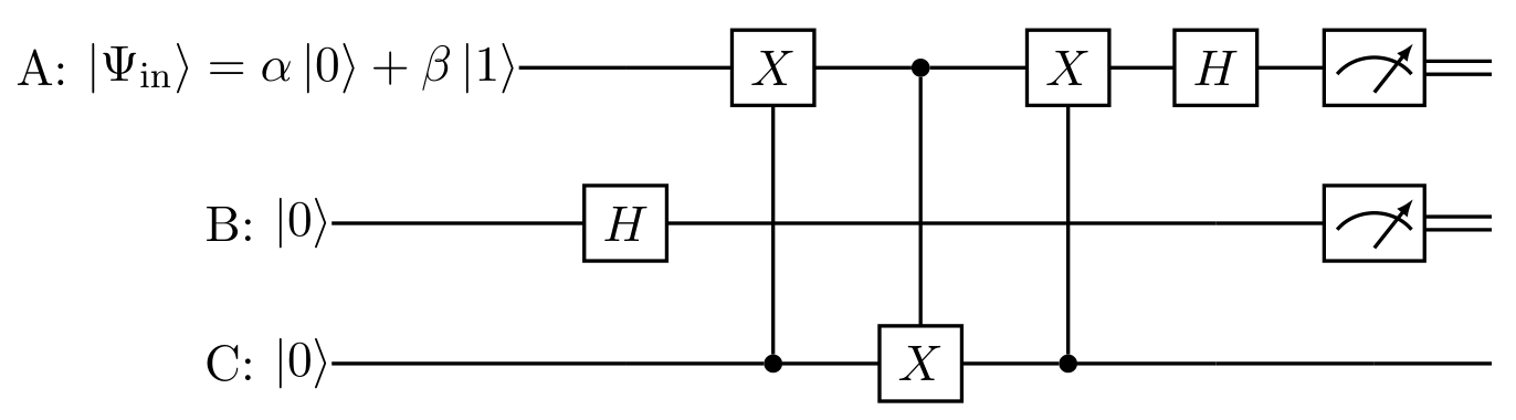
Three alternating CNOT gates is equivalent to the SWAP gate, so we can write:
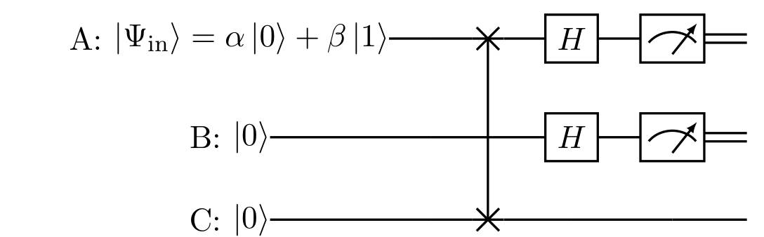
where we clearly see a swapping that occurs between the top and bottom branch!
Building Quantum Computers
According to theoretical physcist David P. Divencenzo, there are five necessary (but not necessarily sufficient) criteria to build a quantum computer:
- A well-characterized qubit.
- The ability to initialize qubits.
- Long and relevant decoherence times.
- A “universal set” of quantum gates.
- The ability to measure qubits.
In this section, we will focus on how we can create qubits and how we can create a universal set of quantum gates. Consider two energy levels as the qubit states respectively. Assume that
Also assume that the qubit state is time varying, in the form of:
i. (14 pts.) Using the above setup, show how we can implement the quantum gates . Hint: The Schrodinger Equation tells us
where .
Published organizer clarifications — separately quoted from the original clarification document, page 2:
- There is a typo in 5c). The output state should be instead of
- The written Hadamard gate should have a factor of in front of the matrix, in order to preserve magnitude.
- 5i) By “implement,” please think about how you would create the gates (or create the same effects as the gates) as a physical system. It’s the real world you’re dealing with here, not just some math!
- Overall Hint: Don’t overthink too much! All that is required for these questions is basic linear algebra (matrices and understanding of basis vectors) and calculus with ordinary differential equations.
Решение
Внимание: Непълно решение
The original key supplies a complete printed grading scheme, with labels (a)–(j) rather than the question’s (a)–(i), but no full proofs or physical implementations. Its grading labels and scores are retained literally.
Grading Scheme
a.
(0.5 pts)
b.
Three answers were acceptable due to question ambiguity:
(i) (0.5 pts)
(ii) (0.5 pts)
(iii) (0.5 pts)
c.
(1 pts)
d.
(1 pts) Drawing/describing the below or equivalent:
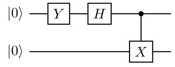
To check equivalent, use website.
e.
(1 pts) Via either matrix multiplication or circuit analysis (or equivalent)
Note: The last step is the trickiest (where you have to deal with measurement, resulting in 4 cases). Make sure the participant checks all 4 cases or uses a clever method to cirumvent checking the cases. If they skip over the measurement step (or it’s not clearly written), deduct 0.5 pts.
f.
(1 pts) Recognizing that classical bits need to be communicated via control wires so the qubit isn’t teleported faster than light.
(1 pts) Stating that nothing can be recovered from the state before classical bits are communicated.
(1 pts) Proving the above statement. (This actually turns out to be much harder, so if the team attempts to prove the above, then give the point. The main idea is to recognize that simply stating you need control wires to prevent FTL communication is not sufficient)
g.
(2 pts) Complete proof. Partial proofs will receive 1 point.
h.
(1 pts) Complete proof. Partial proofs will receive 0.5 points.
i.
(1 pts) Complete proof. Partial proofs will receive 0.5 points.
j.
- (1 pts) Sets up the system of ODE
- (2 pts) Solves the ODE
- (6 pts) Recognizes that the solution can be written in terms of Pauli matrices,
- (5 pts) Shows how using the above form, we can create the gates.
Organizer clarification document — other notes
Separately quoted from the organizer clarification document:
Other Notes
- You are allowed to refer to Wikipedia (but not any other sources). You should typically rederive proofs instead of citing them.
- Uploading images: View this link to find how to upload images on overleaf.
- You are allowed to mix LaTeX and handwritten PDFs for your answer sheet. Note that you need to write your solution to the problem alongside your final answers. If you desire a LaTeX template, we have made one for you here. Make a copy of the project to edit the document.
- You can use basic formulae related to topics on the IPhO syllabus without derivation but all other formulae which go beyond that must be derived.
- If you find that space is running out on your LaTeX file, try to use and see if that fixes it.
Оригинал в Архива: theory.pdf · официални решения: theory_sol.pdf · допълнителни данни: Clarifications.pdf