OPhO 2023, Теория — Задача 2. T2: The Complex Potential
2023 Online Physics Olympiad: Invitational Contest — Theoretical Examination · 5 август 2023 г.
Sponsors
This competition could not be possible without the help of our sponsors, who are all doing great things in physics, math, and education.
Instructions for Theoretical Exam
The theoretical examination consists of 3 long answer questions and 160 points over 2 full days from August 5, 0:01 am GMT.
- The team leader should submit their final solution document in this google form.
- If you wish to request a clarification, please use this form. To see all clarifications, view this document.
- Participants are given a google form where they are allowed to submit up-to 100 megabytes of data for their solutions. It is recommended that participants write their solutions in LaTeX. However, handwritten solutions (or a combination of both) are accepted too. If participants have more than one photo of a handwritten solution (
jpg, png, etc), it is required to organize them in the correct order in apdfbefore submitting. If you wish a premade LaTeX template, we have made one for you here. - Since each question is a long answer response, participants will be judged on the quality of your work. To receive full points, participants need to show their work, including deriving equations. As a general rule of thumb, any common equations (such as the ones in the IPhO formula sheet) can be cited without proof.
- Remember to state any approximations made and which system of equations were solved after every step. Explicitly showing every step of algebra is not necessary. Participants may leave all final answers in symbolic form (in terms of variables) unless otherwise specified. Be sure to state all assumptions.
Problems
- T1: Booster
- T2: The Complex Potential
- T3: General Relativity
List of Constants
| Proton mass | |
|---|---|
| Neutron mass | |
| Electron mass | |
| Avogadro’s constant | |
| Universal gas constant | |
| Boltzmann’s constant | |
| Electron charge magnitude | |
| 1 electron volt | |
| Speed of light | |
| Universal Gravitational constant | |
| Acceleration due to gravity | |
| 1 unified atomic mass unit | |
| Planck’s constant | |
| Permittivity of free space | |
| Coulomb’s law constant | |
| Permeability of free space | |
| Stefan-Boltzmann constant |
Условие
A Conformal Transformation
A complex number can be thought of as a mathematical object that ”stores” two real numbers. An element of the set of complex numbers can be written as:
where is called the imaginary unit, and . With this, one can think of constructing complex-valued functions – namely, a function :
Since complex numbers encode two real numbers and , we can consider complex-valued functions yielding two real-valued functions and that depend on . and , being real-valued multivariable functions, allow us to extend calculus on to . You are given that the composition of two complex differentiable functions yields another complex differentiable function on the appropriate domain.
(a) Starting from the definition of a derivative in single-variable calculus, show that if given in (1) is complex differentiable, and satisfy:
(b) Show that and are solutions to the 2D Laplace equation:
(c) A parametrized curve on the complex plane can be thought of as a function that takes a real number and yields a point on the complex plane. Two parametrized curves and intersect at some point ; tangent lines of the two curves at form an angle . Show that the tangent lines of the curves and at form the same angle , where is the composition function.
A Conformal Transformed Electrostatic System
We know from electrostatics that in a charge-free region, the electrostatic potential satisfies the Laplace equation . As you’ve shown above, this motivates the idea of defining a complex differentiable function whose real part is the electrostatic potential – complex differentiability encodes the fact that the electrostatic potential satisfies (2). Given a 2D electrostatics problem in a charge-free region, we define the complex potential as:
where is an appropriate real-valued function that satisfies the conditions derived in question 1, making a complex differentiable function. You are given the uniqueness theorem: the 2D Laplace equation has a unique solution that satisfies specified boundary conditions.
(d) Given a 2D electrostatics problem and an appropriate complex potential , write the derivative in terms of the and components of the electric field: .
(e) Show that the function satisfies the 2D Laplace equation with the boundary condition while .
(f) The complex logarithm function is defined at as for , . Show that the upper-half plane (points on the complex plane with a positive imaginary part), under the logarithm map, turns into a strip bounded by and . You may assume that the logarithm function is complex differentiable on and that its inverse is for this problem.
(g) Starting from the electrostatic potential in (e), find the electrostatic potential in the region between two infinitely large capacitor plates separated by distance . Carefully argue why this method yields the correct solution.
(h) Show that the function maps the unit circle , centered at the origin, to the real line and the interior of the circle to . Determine the inverse of the function and explain why there’s a one-to-one correspondence between points bounded by and .
(i) Find the electrostatic potential in the region between an infinite rod of charge density and a grounded concentric conducting cylindrical shell of radius .
(j) Now consider the same infinite rod suspended above a grounded conducting plate at a height . Use your results for questions (h) and (i) to derive the electrostatic potential in the region above the plate.
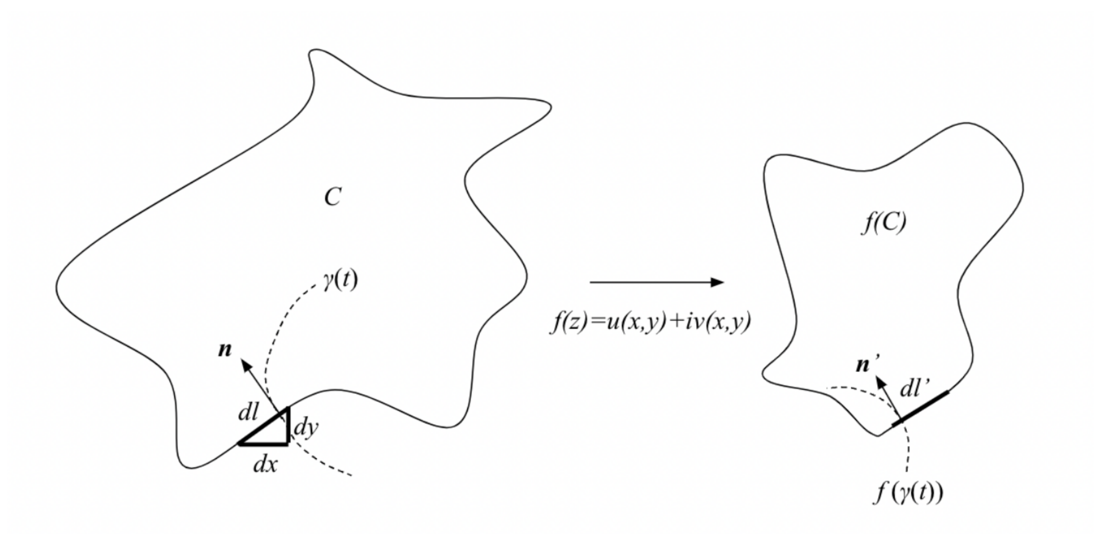
(k) Consider the curve shown in the figure below. You are given that the image of is . If we take some line element on the curve , find the scaling factor to its image on . This is known as a conformal transformation in which the mapping is a holomorphic function.
(l) Take to represent a conductive surface. If is an appropriate solution to the 2D Laplace equation satisfying , find expressions for the surface at , the electrostatic potential satisfying , and the surface charge at from .
(m) Verify that your results for questions (k) and (l) are consistent.
On the Electrostatic Interaction between a Line Charge and a Conducting Wedge
We can apply the knowledge we have gained here to solve a familiar physical puzzle. This puzzle has been widely known and popular in specific cases (e.g. easily solvable using the image method), but it lacks generality. Consider a grounded, infinitely large, conducting wedge with an opening angle . Inside the wedge, there is a thin, infinitely long, straight line with a uniform charge density of per unit length, positioned parallel to the edge of the wedge. The distance between the line and the edge is , the plane that pass through both the line and the edge make an angle with a face of the wedge.
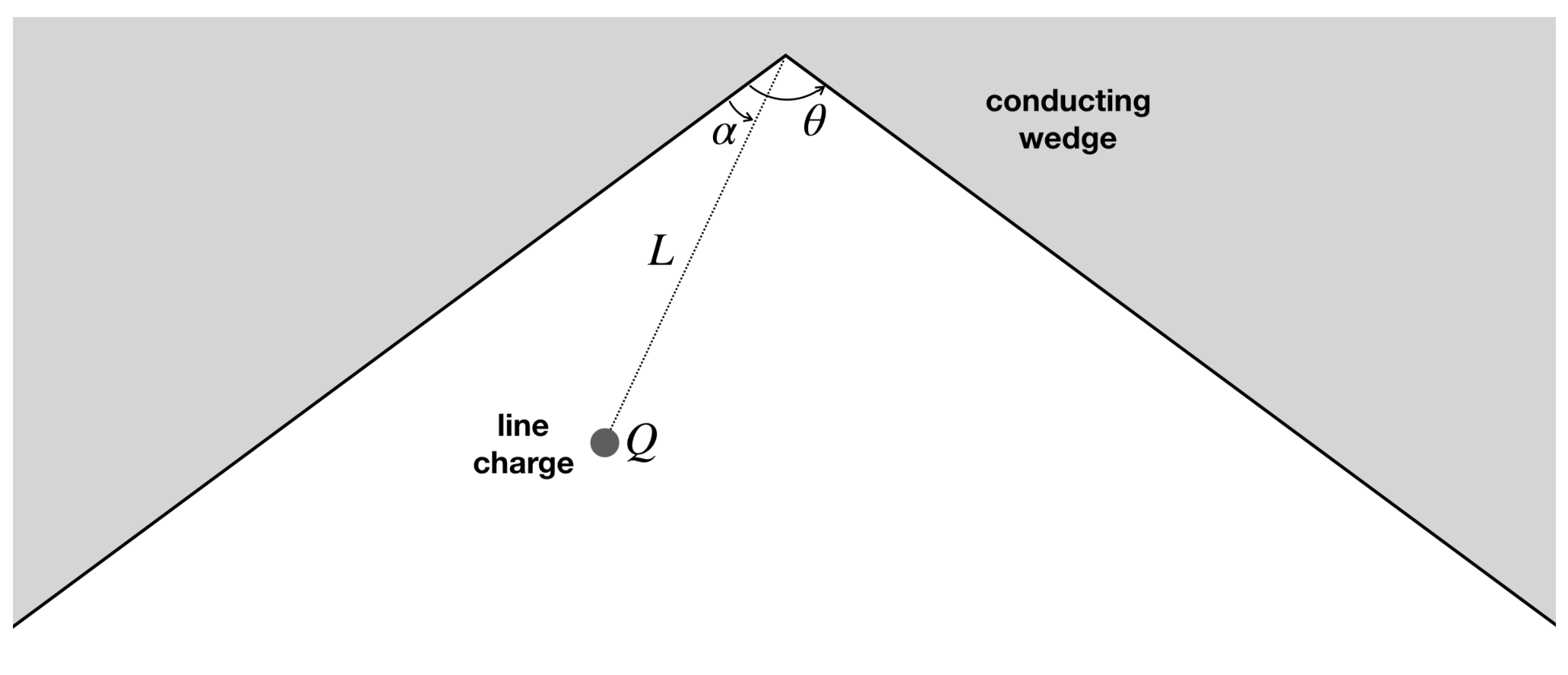
(n) Find the direction and the magnitude of the electrical force acting on the line per unit length. Solve for the general case of , then evaluate your answer in the unit of , for and .
Отговори
A Conformal Transformed Electrostatic System, (d)
A Conformal Transformed Electrostatic System, (g)
A Conformal Transformed Electrostatic System, (i)
A Conformal Transformed Electrostatic System, (j)
A Conformal Transformed Electrostatic System, (k)
On the Electrostatic Interaction between a Line Charge and a Conducting Wedge, (n)
Magnitude for θ = 120°, α = 30°.
Решение
Solution 2:
Part A
Has hinted in the problem, we define differentiability of complex functions just as we would in single variable calculus on the reals. A function , is complex-differentiable or holomorphic at a point if the following limit converges to a number :
We call the number the derivative of at . Note that the limit is taken by any sequence of points in the complex plane that converges to the origin. As in multivariable calculus on , can approach the origin in two different ways: along the real axis and along the imaginary axis – both limits should yield the same result if the limit in (1) indeed converges. If moves along the real axis, . The limit in (1) becomes:
where . If we write , the limit then becomes:
but we see that these are just partial derivatives evaluated at :
Now, if we move along the imaginary axis, . The limit in (1) becomes:
Following a similar procedure from before:
Since , the limit can be written as:
As discussed, if is complex-differentiable at , these limits should be equal. Equating real and imaginary parts, we find:
Part B
From the conditions in (2), we observe that:
It can similarly be shown that . We therefore find that a holomorphic function has real and imaginary parts that satisfy the 2D Laplace equation.
Part C
The ‘tangent vectors’ along at and at are represented by the complex numbers and , respectively. Let us denote the ‘dot product’ of two complex numbers and as: . The cosine of the angle is therefore:
The transformed curves and , at the intersection , will have tangent vectors and , respectively. Let us write for and . Using the chain rule,
And similarly for :
Now, let us consider the cosine of the angle formed between and :
Denoting the derivatives with dots and omitting the input points/parameter values,
Hence,
Note that since is complex-differentiable, we require . Applying the condition found in (a) to the second term, we find that it vanishes. Hence,
Now, observe that and
As was to be shown.
Part D
Note that for a holomorphic complex potential , taking the derivative in the real direction:
was chosen such that so
Part E
There was a domain issue in the original problem statement – should be added/subtracted depending on the domain, but this shouldn’t matter in verifying the 2D Laplace equation since it involves derivatives. A better statement would be for , which clearly satisfies the given boundary conditions , . In spherical coordinates, the Laplacian operator is
Hence,
By the uniqueness theorem, the true, unique electric field respecting the boundary conditions is modeled by .
Part F
A radial line on the upper half plane at angle is the set of points . Under the logarithm map, this set is mapped to which is clearly the horizontal line at extending . Since the upper half plane can be thought as the collection of the sets for , is clearly the strip bounded by and . Let us call this strip . We are given that is holomorphic on and that
Part G
Note that the boundary condition in (e), under the logarithm map, becomes the desired boundary conditions of two infinite capacitor plates. Let us crudely denote the ‘potential space’ as – the space to which complex potentials map. For example, if is an appropriate complex potential to (e), we may write with the boundary condition and defined on the upper half plane . We observe that taking a map defines a complex potential with the boundary conditions and defined on . For an arbitrary separation , we can consider . Since and are holomorphic, so is . As verified in (b), this means that the real part, , satisfies the 2D Laplace equation, as well as the boundary conditions and , hence a valid potential for this problem. We have:
for . This is indeed the expected result from basic electrostatics.
Part H
This problem really isn’t approachable without rigorous mathematical reasoning. The unit disc is the set defined by . The upper half plane is defined by the set . We first show that . For any , we observe that
Clearly, if , we have
implying . Since for an arbitrary we have , . Now we’d like to show that . Consider an arbitrary . We’d like to show that there exists a number such that , which would imply . Observe that:
Now, note that , so when comparing and , we need only compare the imaginary parts. Denoting ,
since , we can get rid of the absolute value symbol – – and make the above a strict inequality. This suggests that , which implies , and we conclude:
so for all , there exists a with . We’ve shown that and that , implying . The way we found above hints that the , pair is defined uniquely – that there is a one-to-one correspondence such that is bijective. To show this, we can first suppose that has an inverse defined by:
is clearly single-valued, and it’s easy to verify that and . This would be a direct proof that is a bijection between and . Now we observe the mapping of the circle . Note that there should be problems with around since is not holomorphic at . For an arbitrary point with , it’s easy to simplify expressions down to:
Graphing this on desmos suggests that the arc maps to the positive real line and that maps to the negative real line. Notice there’s a jump from to as we move from the top arc to the bottom arc at – this is where “breaks”.
Part I
This is a standard electrostatics problem. The potential in the region between the rod and the cylindrical shell can be found by integrating the appropriate electric field .
where is the radius of the concentric cylindrical shell.
Part J
From our results in (h), let us define a map , where is the disc of radius centered at the origin, as:
Under this map, the set up in (i) is mapped to the boundary conditions on : on the real line, infinite rod placed at . These are the exact boundary conditions that we require for this problem. The inverse map of , denoted , is given by:
is holomorphic everywhere on the complex plane except at , which isn’t included in , so holomorphic on the upper half plane. Since the boundary condition satisfied by has the geometry of , we can consider a complex potential that maps . As argued in (g), is a holomorphic function on that respects all necessary boundary conditions. Since is only dependent on , we’d like to consider :
If we identify and , the desired potential function is:
A method of images results in the same expression.
Part K
If we parameterize the curve as , the length element at can be written as:
with all derivatives evaluated at . We can use the calculations in (c) to write in terms of :
Hence, we find the scaling factor is .
Part L
If is orthogonal to , the surface charge at is proportional to . Since the surface is a conductor, is parallel to near the surface. From previous problems, we know that is the appropriate electrostatic potential in , and is parallel to the mapping of , which remains orthogonal to the curve, as shown in (c). There’s a theorem that states that if is a bijective holomorphic map, never vanishes, is holomorphic, and the derivative of is given by . However, since we deal with the individual real and imaginary components of complex functions in this question, we may crudely rely on calculus on . The surface charge at is proportional to . Carefully applying the chain rule results in:
Part M
If we take the charge at points to remain the same even after conformal transformations (think about stretching charged surfaces with the charges glued in place) we see that the scale factor found in (j) results in the scaling of the surface charge found in (l). Hence, given that functions behave nicely at boundaries, we can determine the surface charge of other surfaces simply by looking at the form of and its derivative.
Part N
The electrostatic system of interested is effectively two-dimensional. For simplicity, set and . We can recover the general answer with dimensional analysis later on.
Consider a configuration in -space in which the grounded conductor fills the area and a charge is placed at position . This configuration can be mapped to our puzzle in -space by the conformal transformation as shown in the figure below.
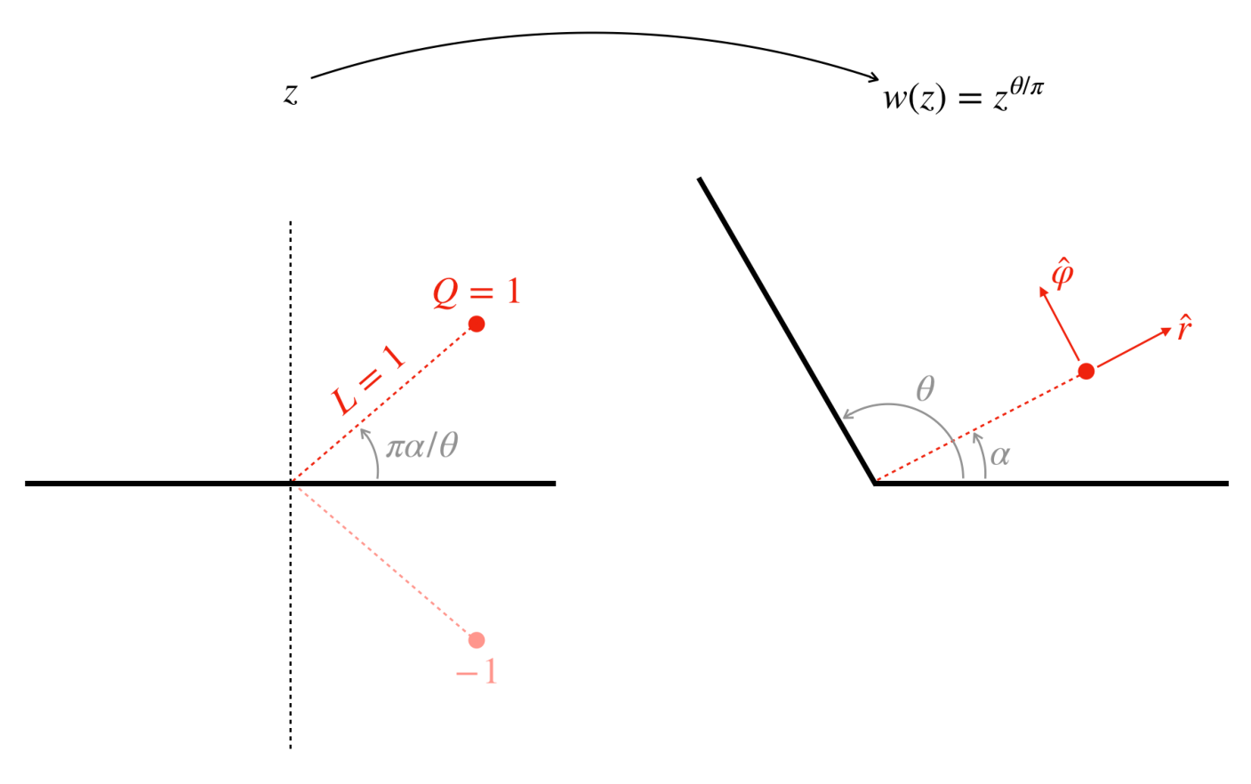
In -space, the electric potential in open space is as if created by the original charge and the image charge located at position . Thus, the complex potential is given by:
After the transformation , in -space it becomes :
Choose a polar coordinate , then we can obtain the real potential as:
Subtract this by the electric potential created by the original charge in the -space, we have a regularized complex potential which is not singular at the location of that charge:
We can then calculate the electrical field created at the location of the original charge by the induced charge distributed on the conducting wedge:
The total electrostatic force acting on the original charge is therefore , and after putting back and , we arrive at the expression:
For and , the magnitude of this force in the unit of is .
* This part was created with helps from Quy C. Tran and Nam H. Nguyen.
Grading Scheme
(a) 1.5 pts
(b) 1.5 pts
(c) 5 pts
(d) 1.5 pts
(e) 1 pt
(f) 1.5 pts
(g) 7.5 pts
(h) 7.5 pts
(i) 1.5 pts
(j) 7.5 pts
(k) 5 pts
(l) 5 pts
(m) 1.5 pts
(n) 15 pts
Оригинал в Архива: theory.pdf · официални решения: theory_sol.pdf