OPhO 2024, Експеримент — Задача 1. Phase Transition
2024 OPhO Experimental Exam: Ising Model of Ferromagnetism · 30 август 2024 г. · 25 т.
Условие
Introduction
Paramagnetic materials have atoms with permanent magnetic dipoles, but point in random directions unless aligned by an external magnetic field. On the other hand, magnetic dipoles in ferromagnetic materials align with neighboring dipoles and can have a significant magnetization even without an external field.
Iron is one common example of a material that is ferromagnetic at room temperature. Other materials undergo a phase transition, where they are paramagnetic at higher temperatures, but become ferromagnetic below a certain temperature (the Curie temperature, ).
In this experiment, we will use the Ising Model and a Monte Carlo simulation to compute and examine the properties of this phase transition.
The Ising Model is a simple approximation for ferromagnetism. We take a 2D lattice of atoms and assume that each dipole points either up () or down () along the same axis. Then we run the Monte Carlo simulation, which uses the following algorithm:
- Start with a 2D grid of size , where each site represents a spin that can be either or . The initial configuration is randomly assigned.
- Energy Calculation: For each spin at position , calculate the change in energy () if the spin is flipped. This is done by considering the interaction of the spin with its nearest neighbors. The energy change (in the absence of an external field) is given by:
where is the interaction strength. 3. For each Monte Carlo step:
- Randomly select a spin in the grid.
- Calculate the energy change if this spin were to be flipped.
- If , flip the spin.
- If , flip the spin with probability , where is the temperature and is the Boltzmann constant.
- Repeat the spin-flipping process for a set number of steps, allowing the system to reach equilibrium.
- The final configuration of the grid after the simulation, representing the state of the system at temperature .
Accessing the Program
To access the Python notebook, follow this link and make a copy to your own Google Drive. You will be able to perform all the code online without needing to download anything.
Overview of Code
There are three cells to run experiments:
- Varying the temperature via
T_listwhich contains all of the simulated temperatures. - Varying the external magnetic field via
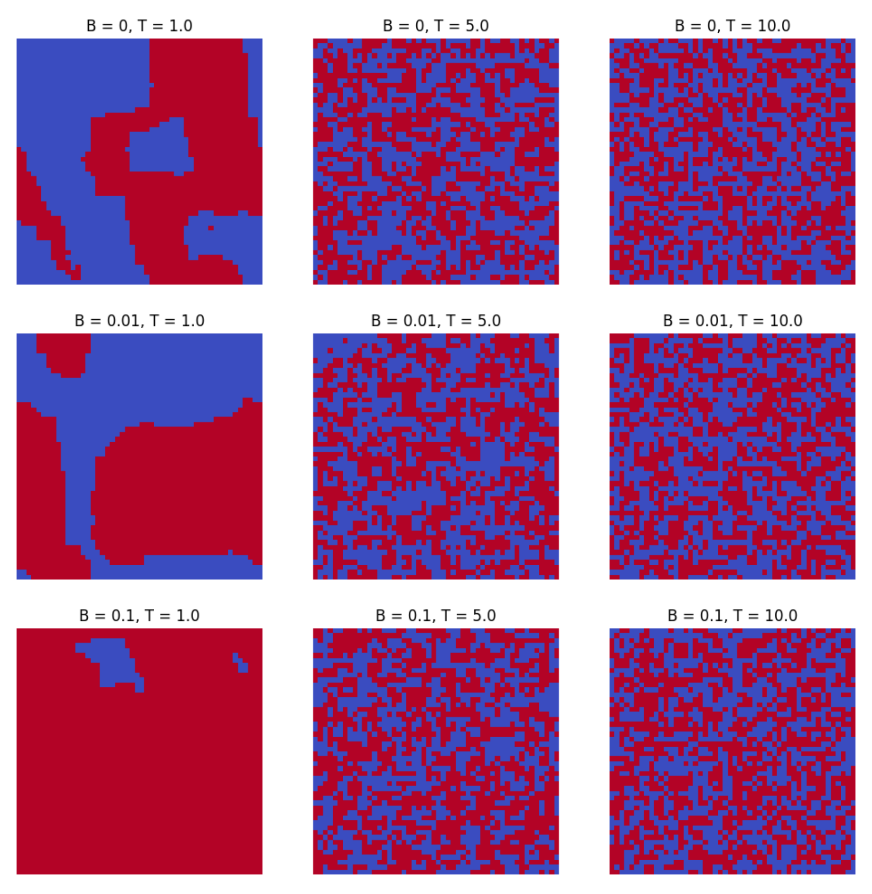
B_listwhich contains all of the simulated external fields. - Varying both.
Instructions for Using the Simulation
- The simulation uses a 50x50 grid to represent the 2D lattice of atoms. This grid is periodic, meaning that it wraps around at the edges, allowing for continuous boundary conditions.
- You can simulate the system at different temperatures by adjusting the
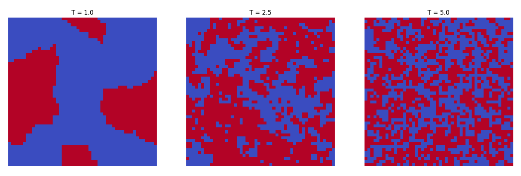
T_listorB_listvariable (based on desired experiment) in the code. The default temperatures provided are 1.0, 2.5, and 5.0. - The number of Monte Carlo steps can be modified by changing the
n_stepsvariable. The default is set to 100,000 steps, but you may increase or decrease this based on your needs. - The interaction strength (
J) and Boltzmann constant (k_B) are set to 1.0 by default. It is recommended not to change these values as they are critical to maintaining the accuracy of the model. - Once you’ve adjusted the parameters, run the cells in the notebook to simulate the Ising Model at the chosen temperatures. The results will be visualized, showing the spin configuration of the grid for each temperature.
Below is an image of what the initial simulation should look like for the first cell:
For the second cell:
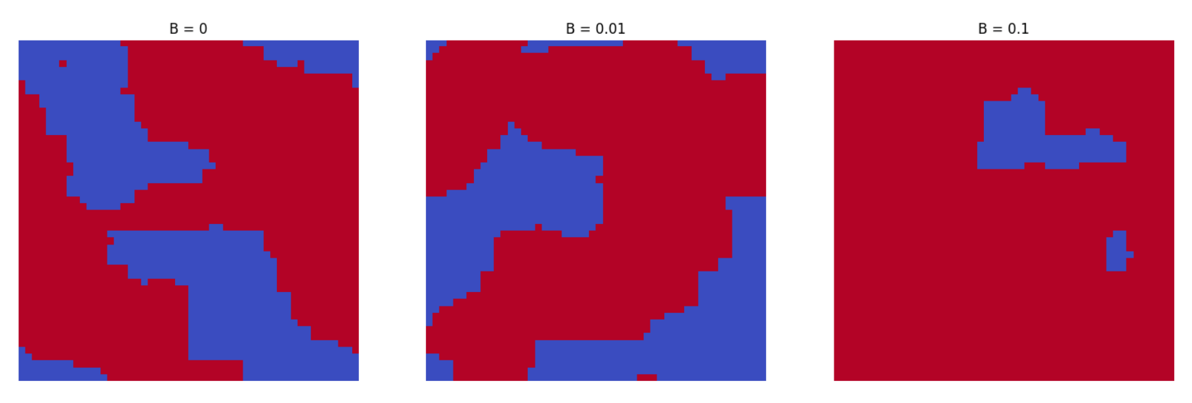
For the third cell:
Phase Transition
For the following questions, include the figure with uncertainty if applicable, your reasoning, and any graphs if used.
a) Find the value of and explain what criteria you used. [6 т.]
b) Keeping the external magnetic field constant, plot the energy of the system as a function of temperature. [4 т.]
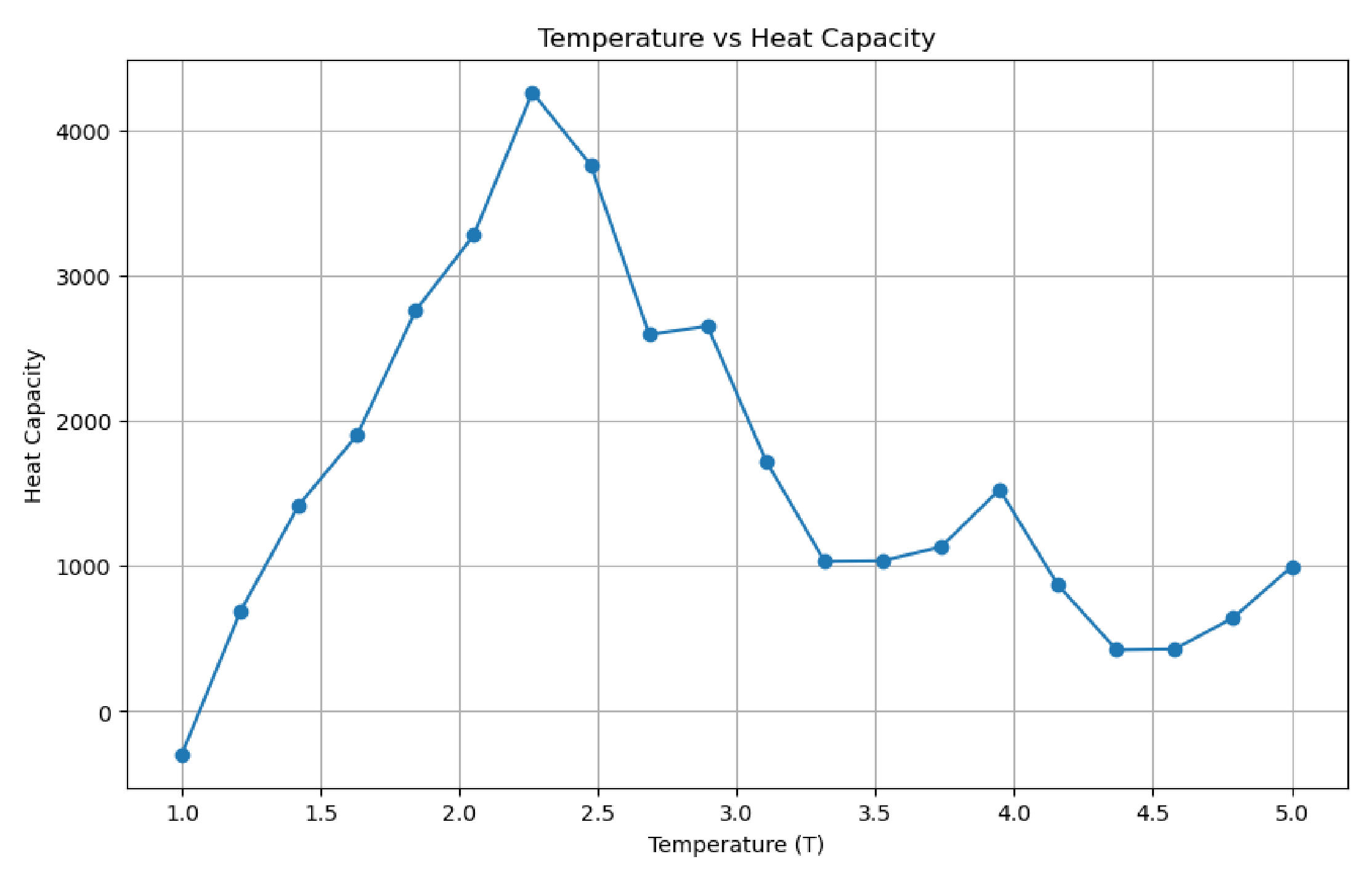
c) Plot the heat capacity of the system as a function of temperature. What are its maximum and minimum values?
A phase transition is first order in temperature if the energy is discontinuous, second order if the energy is continuous but its first derivative is discontinuous, etc. What is the order of the phase transition here? [5 т.]
Consider the net magnetization of the system.
d) At temperatures slightly below , can be approximated as . Find values for and . [6 т.]
e) Set . Plot how the net magnetization reacts as is varied. Qualitatively, what do you observe? What happens if ? [4 т.]
Отговори
a) 2.269
Official marking scheme: Final Answer: .
c) 2nd Order Phase transition
d) 0.125
Value of β only: the official marking scheme gives ; no value for α is printed.
Решение
Phase Transition [25pts]
For the following questions, include the figure with uncertainty if applicable, your reasoning, and any graphs if used.
a) Find the value of and explain what criteria you used. [6pts]
Solution Needs:
- [2pts] Set , vary and plot measures.
- [3pts] Measures of switching from ferromagnetism to paramagnetism:
- (a) Transition of average magnetization oscillates between -1, 1 to tapering at 0.
- (b) Inflection point of absolute value of magnetization.
- (c) Transition between energy to increasing energy.
- [1pts] Final Answer: AND one of the above is scored.
b) Keeping the external magnetic field constant, plot the energy of the system as a function of temperature. [4pts]
Solution Needs:
- [1pts] Correct energy Hamiltonian.
- [2pts] Write code/use method to calculate .
- [1pts] Plot vs. . Look smth like this:
c) Plot the heat capacity of the system as a function of temperature. What are its maximum and minimum values?
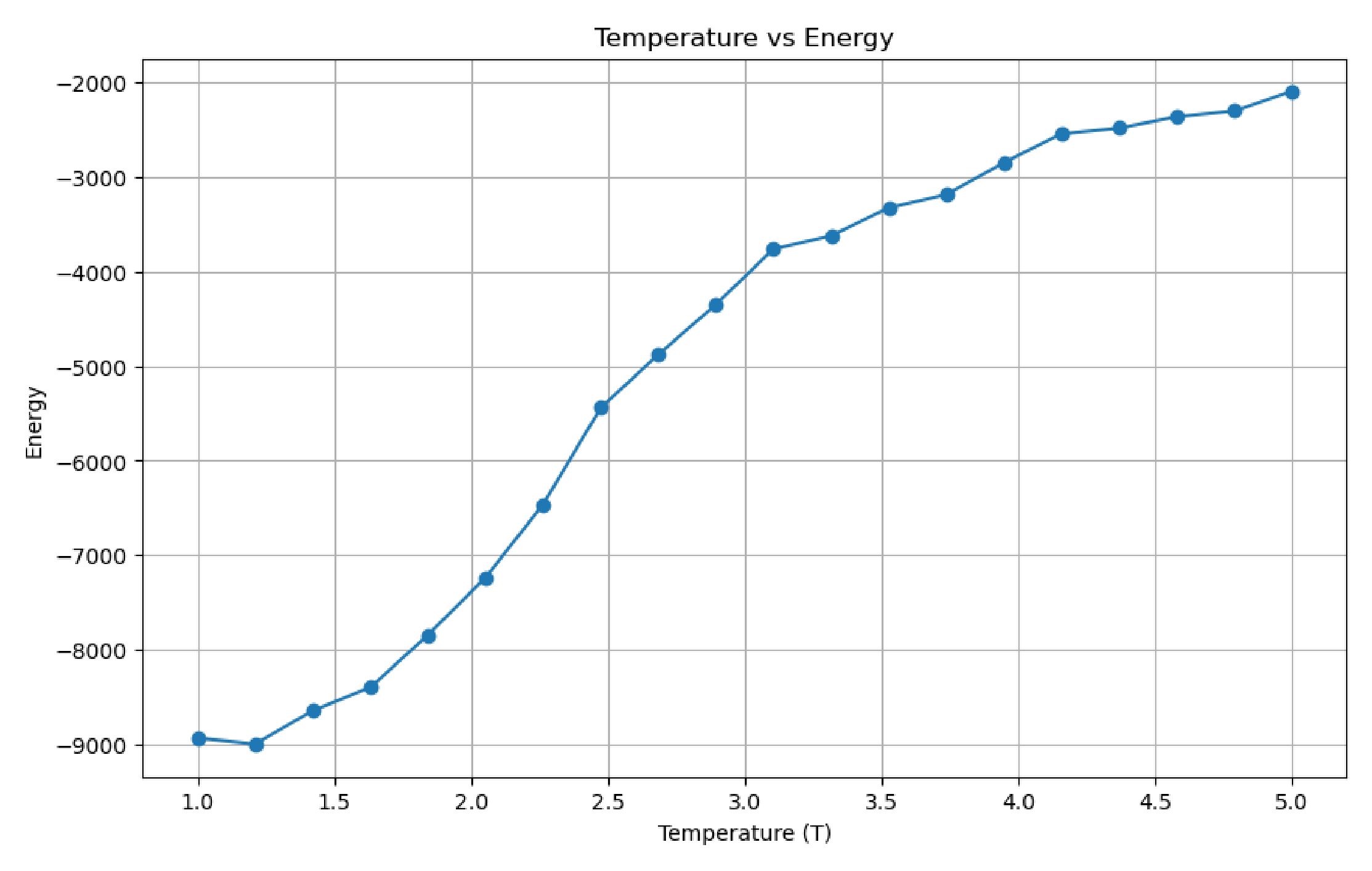
A phase transition is first order in temperature if the energy is discontinuous, second order if the energy is continuous but its first derivative is discontinuous, etc. What is the order of the phase transition here? [5pts]
Solution Needs:
[1pts] Note .
[3pts] Write code/use method to calculate and plot vs. . Look smth like this:
[1pts] Conclude 2nd Order Phase transition.
Consider the net magnetization of the system.
d) At temperatures slightly below , can be approximated as . Find values for and . [6pts]
Solution Needs:
- [3pts] Plot vs. or equivalent.
- [2pts] Fit linear line either via code or fitting.
- [1pts] Conclude AND equivalent steps to above were followed.
e) Set . Plot how the net magnetization reacts as is varied. Qualitatively, what do you observe? What happens if ? [4pts]
Solution Needs:
- [2pts] Plot vs. and make observation.
- [2pts] Plot vs. varying both . Observations may vary.
Оригинал в Архива: experiment.pdf · официални решения: experiment_sol.pdf