Съдържание

OWAO 2025, Практически тур — Задача 3. Beyond the World’s Edge

Оригинал на условието (PDF)Съобщи за грешка

Всички материали от OWAO 2025

ΩWAO 2025 ◇ Practical Round ◇ Problems · 20 т.

Условие

Fractal dimension ( $D$ ) is a fractional value that measures the complexity and roughness of a shape. It describes how a detail-rich structure fills space and often exhibits self-similarity — meaning parts of the structure resemble the whole, at least statistically, when scaled. For example, a perfectly random distribution of points in a plane would have a fractal dimension equal to the dimension of the space itself, $D = 2$ . A value less than 2 indicates a “clumpy” structure with significant empty spaces (voids). The transition scale from a fractal to a homogeneous universe is an active area of research.

The file SN_cat.csv provides observational data for supernova events. The columns are:

sn_name supernova designation;
redshift measured redshift;
gal_type morphological type of the host galaxy;
sn_ra right ascension in hours, minutes, and seconds;
sn_dec declination in degrees, minutes, and seconds.

a) Plot the objects on a rectangular sky map with axes (Right Ascension; Declination) in degrees. Are there any regions without objects? What does the largest such region represent? [6 т.]

For the remainder of the problem, we will only consider a region of the sky

\delta \in [-5^{\circ};\ +5^{\circ}],

\alpha \in [300^{\circ};\ 360^{\circ}] \cup [0^{\circ};\ 60^{\circ}],

where the object sample seems to be complete.

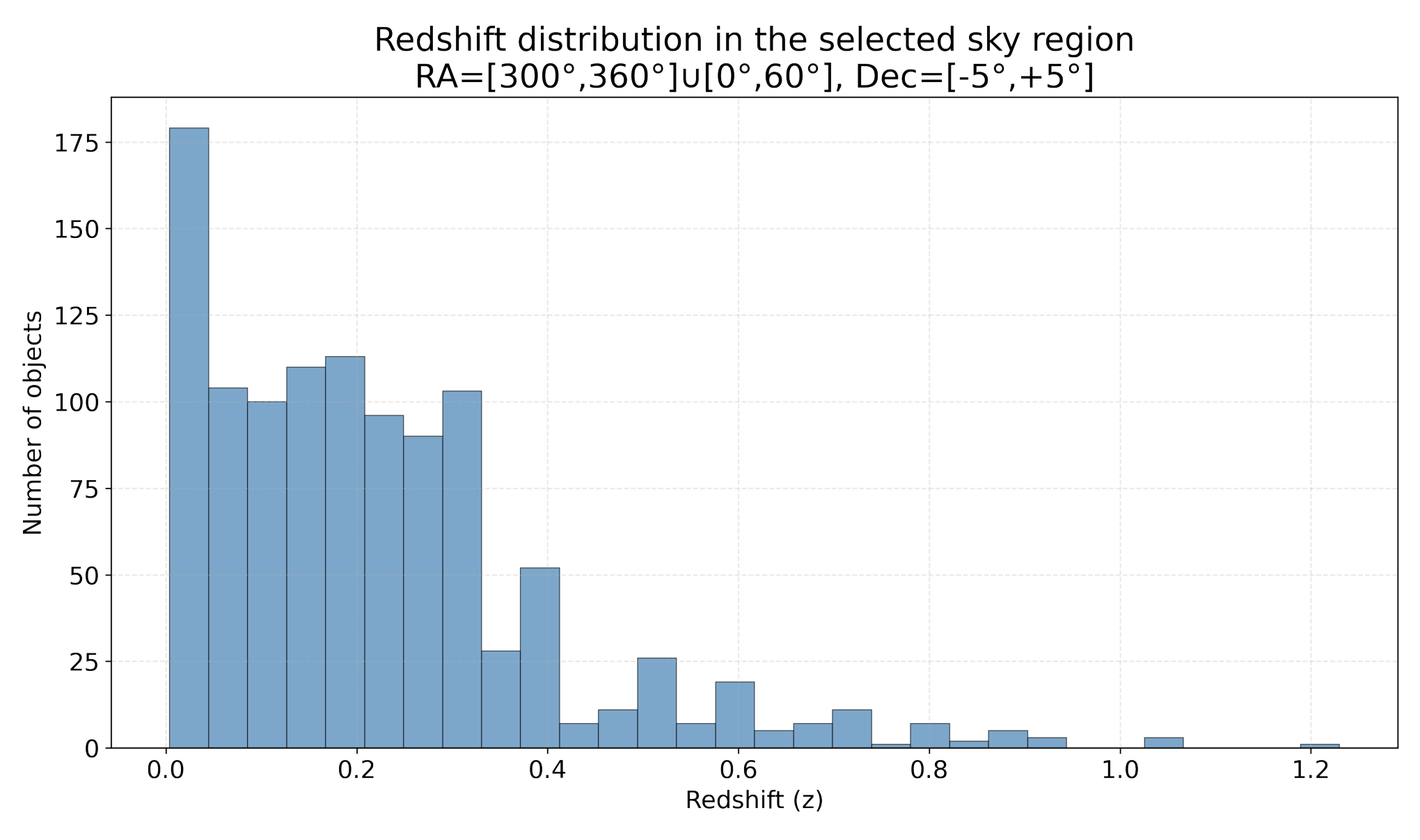
b) For the selected region, plot a histogram of the redshift distribution. [5 т.]

Keep only objects with redshift $z \leqslant 0.1$ .

For these objects, we will determine the fractal dimension. To do this, it is necessary to calculate the pairwise distances $l_{i,j}$ for all pairs $(i, j)$ of the remaining objects. The redshift is small — use ordinary Euclidean distance without applying cosmological models.

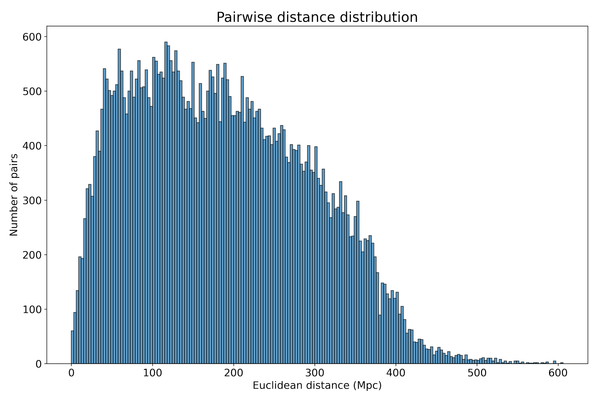
c) Plot a histogram for the distribution $f(l)$ of pairwise distance values. [5 т.]

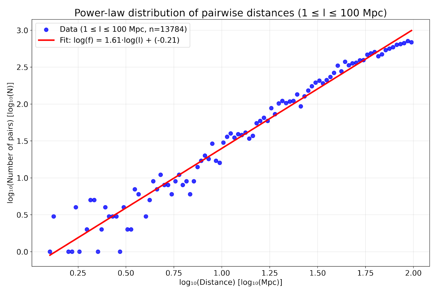
d) To determine the fractal dimension, use pairwise distances $l$ in the range from 1 Mpc to 100 Mpc. Fit the distribution with a power law $f(l) = A\,l^{D}$ . [2 т.]

The sample objects populate an oblate, practically 2D-region. Therefore, $D$ is the fractal dimension of the two-dimensional projection. We may use Mandelbrot’s empirical rule to estimate the fractal dimension $D_0$ of the spatial (3D) distribution of supernovae: $D_0 = D + 1$ .

e) Write down the obtained value of $D_0$ . Is $D_0$ greater or less than 3? [2 т.]

Отговори

Решение

Solution

a) We first convert the right ascension from hours to degrees (using the factor $15^{\circ}$ per hour), and then plot the supernovae on a rectangular sky map. As customary in astronomy, right ascension increases from right to left.

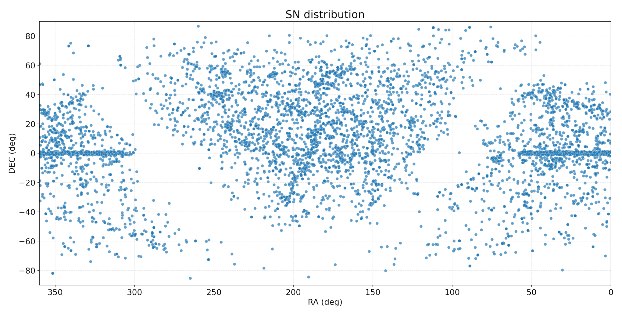
Scatter plot titled “SN distribution”: DEC (deg) from −80 to 80 versus RA (deg) from 350 to 0 (increasing to the left); thousands of supernovae with a broad V-shaped empty band (the Galactic plane) around RA 60–100° and 250–300°, and dense horizontal strips at DEC ≈ 0 near RA 300–360° and 0–60°.

A broad V-shaped band with almost no objects is clearly visible. This feature corresponds to the projection of the Galactic plane onto the celestial sphere. Because the Galactic disk contains large amounts of gas and dust, light from extragalactic supernovae is absorbed, and distant sources in this region remain unobservable.

b) The selected sky region contains a total of 1090 supernovae with redshifts in the range $0.00385 \leqslant z \leqslant 1.23000$ . The corresponding distribution (Fig. 2) shows a sharp decline in the number of detections for $z \gtrsim 0.4$ .

Histogram titled “Redshift distribution in the selected sky region, RA=[300°,360°]∪[0°,60°], Dec=[-5°,+5°]”: Number of objects (0–175) versus Redshift (z) from 0.0 to 1.2; the first bin near z = 0 reaches about 179, bins up to z ≈ 0.35 hold about 90–113, then counts drop sharply beyond z ≈ 0.4. — Figure 2: Redshift distribution of the objects

c) After applying the redshift cut ( $z \leqslant 0.1$ ), the sample is reduced to 329 objects. Although this number may seem modest, it already yields $329 \times 328/2 = 53\,956$ pairwise distances for statistical analysis.

At such low redshifts, distances are estimated from the velocitydistance relation:

d = \frac{v}{H_0}, \qquad v = cz.

The pairwise separations $l_{i,j}$ are then obtained using Euclidean geometry. The angular separation $\theta_{i,j}$ follows from the spherical law of cosines:

\cos\theta_{i,j} = \sin\delta_i \sin\delta_j + \cos\delta_i \cos\delta_j \cos(\alpha_i - \alpha_j).

Finally, the spatial separation is given by the planar law of cosines:

l_{i,j} = \sqrt{d_i^2 + d_j^2 - 2d_i d_j \cos\theta_{i,j}}.

The resulting distribution (Fig. 3) rises up to $\sim 50$ Mpc and declines thereafter. This behavior reflects both the finite size of the sample and observational selection effects.

Histogram titled “Pairwise distance distribution”: Number of pairs (0–600) versus Euclidean distance (Mpc) from 0 to 600; counts rise steeply to about 540 near 50 Mpc, stay around 450–590 up to about 250 Mpc, and decline to near zero beyond 450 Mpc. — Figure 3: Distance distribution of the objects

d) Within the range $1 \leqslant l \leqslant 100$ Mpc we find 13 784 pairwise distances. To estimate the fractal dimension we fit their distribution with a power law. It is convenient to work in logarithmic form:

\log_{10} f(l) = D \cdot \log_{10} l + \log_{10} A.

The coefficients can be obtained by least-squares regression applied to the binned histogram values. We adopt 100 bins, which is consistent with the heuristic choice $\sim \sqrt{N}$ for $N \approx 13\,784$ . The resulting distribution on logarithmic axes is shown in Figure 4, together with the best-fitting straight line.

Log–log plot titled “Power-law distribution of pairwise distances (1 ≤ l ≤ 100 Mpc)”: log10(Number of pairs) [log10(N)] from 0.0 to 3.0 versus log10(Distance) [log10(Mpc)] from 0.25 to 2.00; blue data points (legend: Data (1 ≤ l ≤ 100 Mpc, n=13784)) follow a red straight line (legend: Fit: log(f) = 1.61·log(l) + (-0.21)). — Figure 4: Linear approximation of the pairwise distance distribution function in logarithmic axes

Important remark. When constructing a histogram for logarithmic analysis, the binning must be uniform in $\log l$ , and logarithm of bin counts is taken. Applying logarithms to counts from linearly spaced bins produces a biased slope, since the data points are not uniformly distributed along the $x$ -axis. Figure 5 illustrates this incorrect approach.

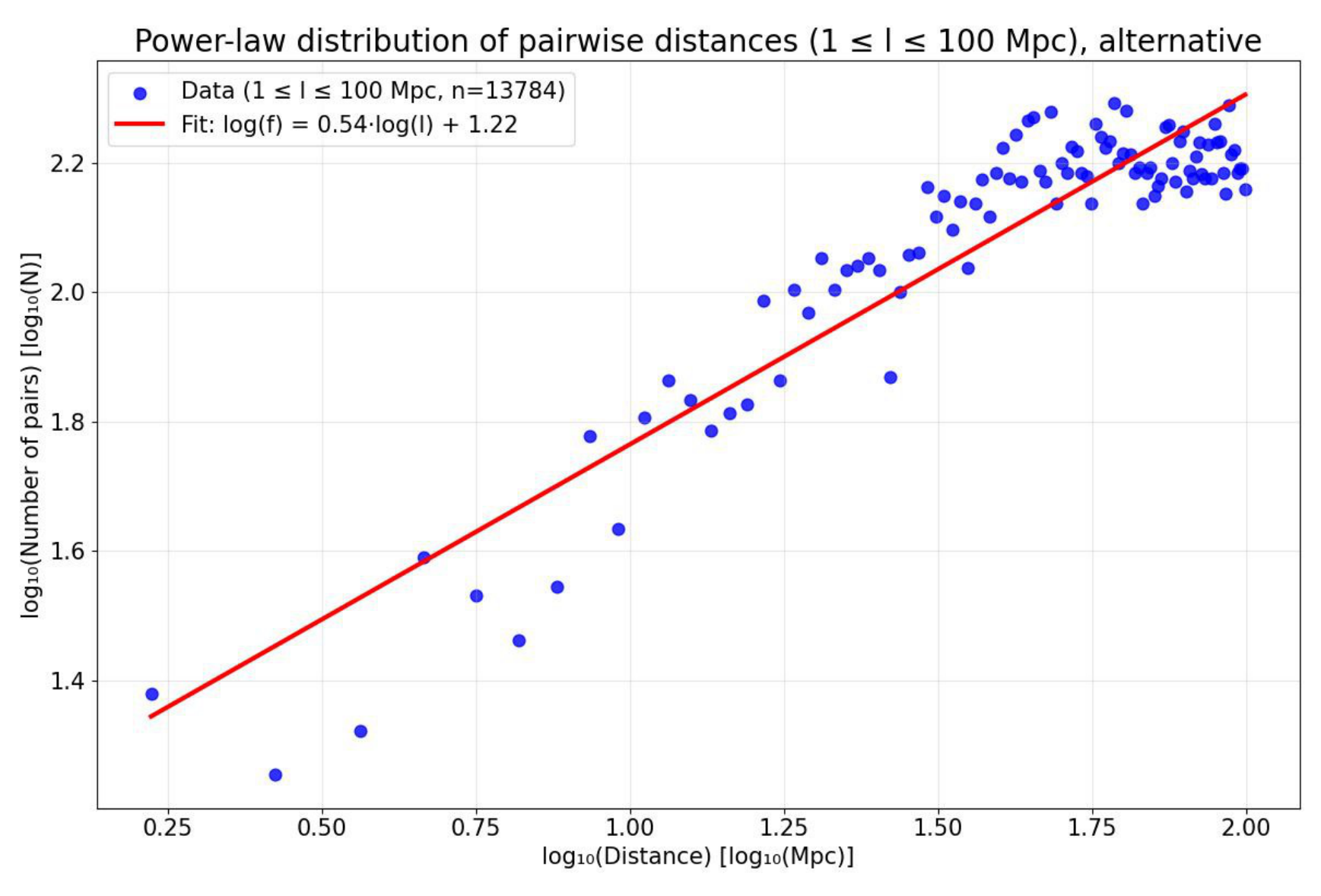
Log–log plot titled “Power-law distribution of pairwise distances (1 ≤ l ≤ 100 Mpc), alternative”: log10(Number of pairs) [log10(N)] from 1.4 to 2.2 versus log10(Distance) [log10(Mpc)] from 0.25 to 2.00; scattered blue points (legend: Data (1 ≤ l ≤ 100 Mpc, n=13784)) crowded at large distances with a red fit line (legend: Fit: log(f) = 0.54·log(l) + 1.22). — Figure 5: Incorrect linear approximation of the pairwise distance distribution function in logarithmic axes

From the regression we obtain $D = 1.61 \approx 1.6$ . Using Mandelbrots empirical rule, the inferred fractal dimension of the three-dimensional distribution is

D_0 = D + 1 = 2.6 < 3,

which indicates that the supernova distribution remains structured rather than homogeneous on these scales.

Note 1. The algorithm employed in this problem follows the approach developed by V. Orlov, A. Raikov, and R. Gerasim $^3$ .

Note 2. The fractal dimension of the Universe is not fixed, but depends on the observational scale. On relatively small scales ( $\lesssim 20$ Mpc), the distribution is highly inhomogeneous: galaxies cluster into groups and small clusters, which in turn align along filaments surrounding large empty voids. The resulting “cosmic web” is clearly visible. Here the fractal dimension is well below 3, reflecting the spongy, network-like nature of the structure.

In the intermediate range (20–100 Mpc), we encounter the transition or cross-over scale. As the sampling volume grows, individual filaments and voids are averaged over, the enclosed number of galaxies increases more rapidly, and the fractal dimension rises toward the homogeneous value of 3.

On the largest observable scales ( $\gtrsim 300$ Mpc), the Universe becomes statistically homogeneous. While structure is still present, any sufficiently large region contains approximately the same number of galaxies as any other region of equal size. The effective fractal dimension thus approaches $D = 3$ , indicating that matter fills space uniformly when averaged over such vast scales.

$^3$ See, for example, Raikov, A. A., Orlov, V. V. & Gerasim, R. V. Determination of the Fractal Dimensionality of Large-Scale Structure With Type Ia Supernovae by the Method of Pairwise Distances. Astrophysics 57, 287–295 (2014). https://doi.org/10.1007/s10511-014-9334-9.

Marking Scheme:

Question (a) Distribution on the celestial sphere
1. Correct processing of the initial data — 2 pt.
2. Constructing the supernova map — 2 pt.
  
  Here and elsewhere, “constructing” implies obtaining the final image; providing the code that generates it is not sufficient.
3. Detecting and correctly explaining the void region — 2 pt.
Question (b) Redshift distribution
1. Correct data processing — 3 pt.
2. Constructing the redshift distribution — 2 pt.
Question (c) Pairwise distances distribution
1. Correct calculation of the pairwise distances — 3 pt.
2. Constructing the distribution of pairwise distances — 2 pt.
Question (d) Power law fitting — 2 pt.
Question (e) Result for fractal dimension — 2 pt.

Points are awarded if a correct and well-founded estimate of $D_0$ was obtained.

Константи

Universal

Gravitational constant $G = 6.67 \cdot 10^{-11}\ \frac{\mathrm{m^3}}{\mathrm{kg \cdot s^2}}$
Speed of light $c = 3.00 \cdot 10^{8}\ \mathrm{m/s}$

Astronomical

Astronomical unit $1\ \mathrm{au} = 149.6 \cdot 10^{6}\ \mathrm{km}$
Parsec $1\ \mathrm{pc} = 206\,265\ \mathrm{au}$
Hubble constant $H_0 = 70\ (\mathrm{km/s})/\mathrm{Mpc}$

Emission constants

Stefan–Boltzmann $\sigma = 5.67 \cdot 10^{-8}\ \frac{\mathrm{W}}{\mathrm{m^2 \cdot K^4}}$
Wien’s displacement $b = 2898\ \mathrm{\mu m \cdot K}$

Earth

Radius $R_\oplus = 6371\ \mathrm{km}$
Obliquity of ecliptic $\varepsilon = 23.4^{\circ}$
Orbital period $T_\oplus = 365.26\ \mathrm{days}$

Sun

Radius $R_\odot = 6.96 \cdot 10^{5}\ \mathrm{km}$
Mass $\mathfrak{M}_\odot = 1.99 \cdot 10^{30}\ \mathrm{kg}$
Absolute magnitude $M_\odot = 4.74^{\mathrm{m}}$ (bol.)
Effective temperature $T_\odot = 5.8 \cdot 10^{3}\ \mathrm{K}$
Luminosity $L_\odot = 3.828 \cdot 10^{26}\ \mathrm{W}$

Оригинал в Архива: OWAO_2025_Practical_Problems.pdf · решение от архива: OWAO_2025_Practical_Solutions.pdf