RMPh 2021, Експеримент — Задача 2. Exercise 2: Measure the lifetime of D0
Romanian Master of Physics 2021. Experimental Problem - Measurement of D0 lifetime · 9 т.
Условие
In this exercise you will use the second part of the application called ”D0 exercise”.
The object of this exercise is to use a data sample of about 50000 events to measure the lifetime of the D particle. This is the same quantity as the half-life of a radioactive particle: the D decays according to an exponential distribution, and if this exponential is fitted to a distribution of the D decay times, the slope of this exponential is the lifetime of the D.
Definitions:
After starting the exercise you will be able to draw plots of the data, change ranges of the variables, make fits of the invariant mass and the lifetime of the D0. The following variables will appear in the exercise:
- D mass: this is the invariant mass of the D particle. The signal can be seen as a peaking structure rising above a background. The range of masses relevant for this analysis is 1816-1914 MeV. The signal shape is described by the Gaussian (also known as "normal") distribution. The center ("mean") of this distribution is the mass of the D particle, while the width represents the experimental resolution of the detector.
- D TAU: this is the distribution of decay times of the D candidates. The signal is described by a single exponential whose slope is the D lifetime.
- D0 IP: this is the D distance of closest approach ("impact parameter") with respect to the proton-proton interaction in the event. The smaller the impact parameter, the more likely it is that the D actually came from that primary interaction. In order to simplify the drawing, we actually plot and cut on the logarithm (base 10) of this quantity in the exercise.
- D PT: this is the momentum of the D transverse to the LHC beamline.
Fitting the signals: mass distribution and the lifetime
The application performs the fitting of the signal in two variables the mass of D0 and the lifetime, your choices are to select the ranges of the four variables mentioned above such that you select (and measure) the signal and remove the background events.
To obtain a value for the lifetime you will use the method of background subtraction described below.
- Click on the Plot D mass button to plot the overall mass distribution. You will see a peak (signal) on top of a distribution (background). The peak should be described by a Gaussian function, whose mean corresponds to the mass of the D and whose width (σ) is determined by the experimental resolution of the LHCb detector.
- Click on Fit mass distribution to fit this distribution using a Gaussian function for the signal and a linear function for the background.
- Look at the fitted mass distribution. You can split it into three regions: the signal region and two background-only "sidebands": one above the signal (the upper sideband) and one below the signal (the lower sideband).
- Use the slider labelled Sig range to define the beginning and end of the signal region. All events not falling into the signal region will be said to fall into the background region.
- You can now use the definitions of the signal and background regions in the mass variable to determine the signal and background distributions in other variables. Click on the button labelled Apply cuts and plot variables. You will see the signal (blue) and background (red) distributions for the other three variables plotted next to the mass distribution.
You are also able to fit the lifetime of D0 at any time after you are applying some cuts. For every lifetime fit you make, we call it a measurement. Varying the cuts you can perform more measurements.
Tasks
2.1 Define a range for the D0 mass which should be your ‘signal region’. Comment on the criterion you used. [1,5 т.]
2.2 Perform the fit and obtain the value and the statistical error for D0 lifetime. [0,5 т.]
2.3 In addition to statistical uncertainties, measurements can suffer from systematic uncertainties, caused by a miscalibrated apparatus or an incorrect modelling of the backgrounds. One basic technique for estimating these is to repeat the measurement while changing the criteria used to select signal events. If the result changes significantly when changing the criteria, we know that there is something wrong!
Repeat your fit for the lifetime of the D while varying the maximum allowed D impact parameter. The allowed values range from -4.0 to 1.5 in the original fit. Move this upper value down, at least 10 points and make the plot of the lifetime obtained. The application records these points for you and does the plot. Save the plot (outside the application using ‘print screen’ or ‘snipping tool’, name it 2.3_YOURCODE), it will be required.
It helps to write down in a table the values shown on the screen like this
| IP | t (lifetime) | error (statistical) | |
|---|---|---|---|
| 1 | 1.5 | ... | ... |
| 2 | ... | ... | ... |
| 3 | ... | ... | ... |
| 4 | ... | ... | ... |
| ... | ... | ... | ... |
[1 т.]
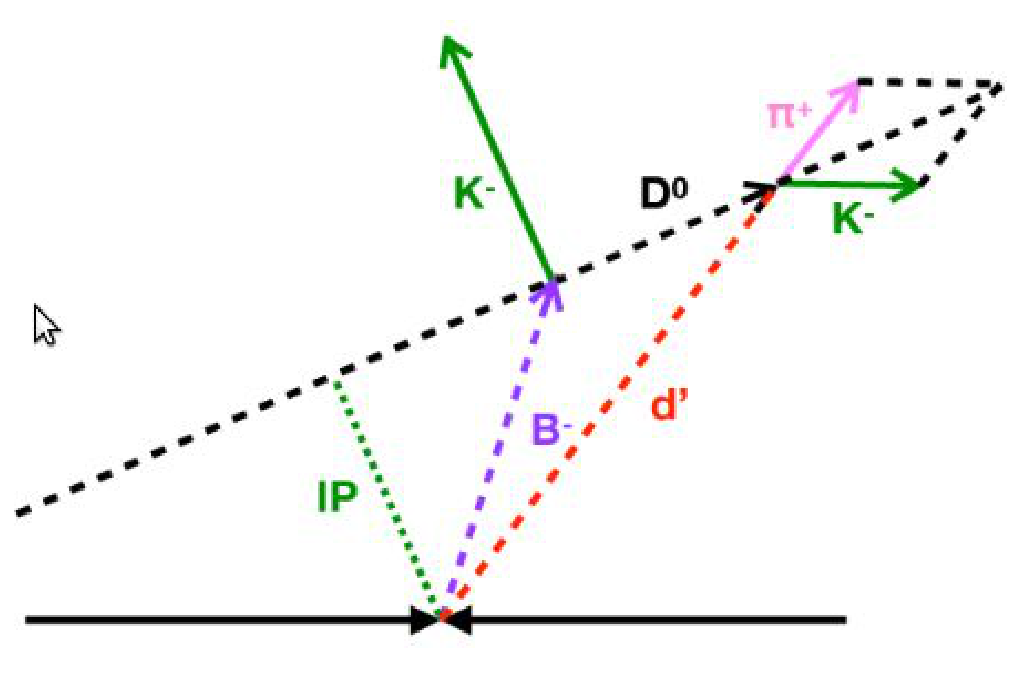
2.4 The sigma-shaped plot you obtained is the indication of the presence of a systematic effect, which once identified can be removed. Make a hypothesis on what causes this systematic effect. [1 т.]
2.5 Seeing the shape of the lifetime as a function of the upper cut on the impact parameter where would you consider to be ‘correct’ value of the lifetime? Give a criterion for where on the plot you would choose this ‘correct’ value to lie. You will do the same thing for the other variables so the criterion should be general to be applied in those cases too. [1 т.]
2.6 Based on the criterion found above choose your best value for D0 lifetime the nominal value, and a range around this point. (Further you will use this range to estimate the systematic error of the measurement). [1,5 т.]
2.7 Repeat the steps 2.3 and 2.6 for the D TAU variable such that you improve the correct value of the lifetime. Create the table suggested above. Making the plot is optional, the application does not perform it. [1 т.]
2.8 Repeat the steps 2.3 and 2.6 for the D PT variable. [1 т.]
2.9 Quote the final value of the D0 lifetime, called the nominal value and the statistical error associated with it. [0,5 т.]
Решение
Exercise 2: Measure the lifetime of D0
2.1 The central value for D0 mass 1866.6, the standard deviations 7.7
A Gaussian distribution contains 99.7% of its events within three standard deviations of the mean, so this "three σ" region around the mean is usually the definition of the signal region.
The range (1843.5, 1869.7) 1,5p
2.2 The value and the fit of the lifetime 0,5p
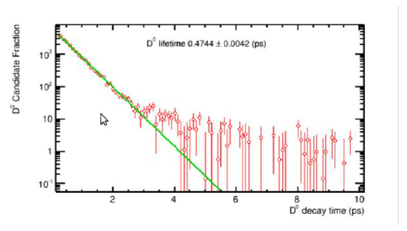
2.3 The plot with two levels 1 p
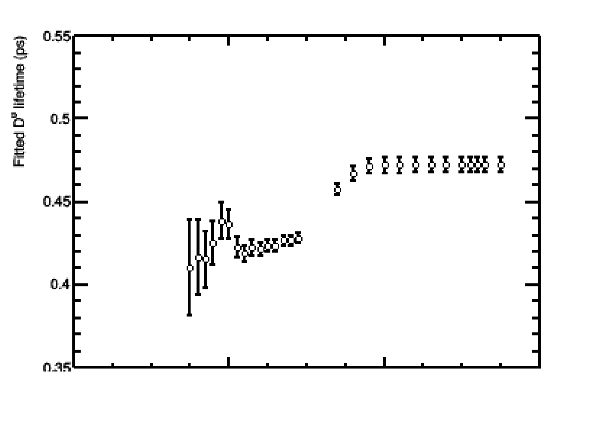
2.4 Hypothesis of another signal coming from another particle with finite smaller lifetime. In this case the B0 mesons. Explaining the possibility of a intermediate decay 1p
2.5 The working region for nominal value, of the D0 lifetime, should be a plateaux or a minimum. The uncertainty of the lifetime by variations around the nominal value should be comparable with the statistical uncertainty for the nominal value. 1 p
2.6 For the IP variable the nominal value should on the lower plateaux in the range (-1.7 , -1.1 )
1,5p
2.7 The measurements for the D0 TAU variable with values similar with the ones below 1 p
| D0 TAU | t (lifetime) | error (statistical) | |
|---|---|---|---|
| 1 | 0,15 | 0,4268 | 0,003 |
| 2 | 0,2 | 0,4212 | 0,003 |
| 3 | 0,25 | 0,4195 | 0,0032 |
| 4 | 0,3 | 0,4159 | 0,0032 |
| ... | 0,35 | 0,416 | 0,0034 |
| 0,4 | 0,4122 | 0,0036 |
2.8 The measurements for the D0 PT variable with values similar with the ones below 1 p
| D0 PT | t (lifetime) | error (statistical) | |
|---|---|---|---|
| 1 | 2,5 | 0,4122 | 0,0036 |
| 2 | 3 | 0,4109 | 0,0041 |
| 3 | 3,5 | 0,4056 | 0,0045 |
| 4 | 4 | 0,3983 | 0,005 |
| ... | 4,5 | 0,4015 | 0,0061 |
2.9 The quotation of the D0 lifetime and the ranges studied before for D0 IP, D0 TAU and D0 PT
0,5 p
Оригинал в Архива: RMPh_2021_Q4.pdf · официални решения: exp_sol.pdf