RMPh 2023, Експеримент — Задача 1. Experimental studies in rotating reference frames
Romanian Master of Physics 2023
Условие
Within the study of all physical phenomena, choosing an adequate reference frame is a mandatory and very important step. Although most of the time the choice is so obvious that we do not even mention it, it is still crucial to be aware of one's assumptions. The main reason:
The laws of physics hold when applied in an inertial reference frame.
Even though the definition of an inertial reference frame might seem a bit circular, and hard to implement in practice (a frame where Newton's law of inertia holds), it yields a very useful characterization:
The relative motion of two inertial reference frames must be translational and uniform.
The real trouble comes when we consider other types of frames' relative motion, which means that at least one of them is non-inertial. When studying non-inertial frames, we simply cannot apply the laws of physics, as we know them. Then, we must resort to one of the following approaches: either reason in an inertial frame, then convert the result to the desired non-inertial frame, or reason in a non-inertial frame, by previously making appropriate changes to the set of laws used.
You should use this second approach with great caution – after all, making changes to the laws of physics is not a job anyone could do! Yet, in some situations, reasoning in a non-inertial frame simply makes more sense. For example, in the case of rotating Earth, if we assume the Sun is an inertial frame, studying Earth's wind currents' flow relative to the Sun would be an unnecessary over complication. You would probably prefer studying this process with respect to Earth, even if it means sticking to a new set of unfamiliar laws. Spoiler alert: by the end of this task, you will get to do exactly this!
Consider the simple case of a uniformly rotating reference frame (with respect to an inertial reference frame). Assume the angular velocity of the rotating frame (with respect to the fixed one) is . Let us study the motion of a point mass moving at position , with velocity and acceleration in the rotating frame. Consider that the net force with which it interacts with other bodies is . Then, it can be shown that our point mass obeys the following equation of motion:
After a simple manipulation, we get:
Notice how similar this expression is to the original Newton's second law. We could interpret the second and third terms on the right-hand side as additional forces acting on our point mass. We call the second one Coriolis force, and the third one centrifugal force.
While apparently "fixing" Newton's second law, this interpretation can lead to confusion when considering Newton's third law - being fictitious forces (that is, just mathematical tricks), the Coriolis force and centrifugal force do not have corresponding equal and opposite reactions!
The additional terms lead to interesting and non-intuitive effects on moving bodies (as viewed in rotating reference frames). In Part A of this problem, you will try to understand their effect by analyzing videos taken in rotating reference frames. In Part B, you will use the previously acquired knowledge to analyze wind.
Part A and Part B are independent. You can solve them in any order.
Part A
In this part of the problem, all processes will be considered in a frame , which is rotating with angular speed with respect to some inertial reference frame. The rotation axis passes through the origin . You must give all answers with respect to the rotating frame.
For the beginning, we will treat the simple case of a non-interacting particle () with mass . Suppose that, at , this point mass is located at , , and , and has velocity . In this case, the equation of motion has the solution
A1 Check that this solution satisfies equation (1). [1 т.]
At small times, close to the beginning of motion, and for a certain range of initial speeds, we may neglect one of the two fictitious forces, so that the trajectory becomes a circle.
A2 1. Which of the two fictitious forces should you neglect to obtain a circular trajectory? 2. Show that in this limit, the two above expressions reduce to a circular trajectory, the radius and center of which you will find. 3. For what range of values (high speeds vs. low speeds) of the initial speed is this approximation suitable? [2 т.]
You will now use this knowledge to solve a puzzle.
You can take videos (of length and frame rate ) in a rotating reference frame, whose rotation speed is unknown. The camera is rotating together with the reference frame. The length scale of these videos is also unknown: you can measure distances on the frames only in arbitrary units of length (a.u.l.). To find these two unknowns, you can perform the following experiment: from a fixed point, at distance from the coordinate system origin, you launch a bead (blue on the video) with speed oriented towards the origin. The origin is marked by a red dot on the videos, and the axis of rotation passes through it, perpendicular to the image plane.
You can launch the bead using either of two cannons. Cannon 1 has adjustable initial speed (in cm/s), in the range [5, 30] cm/s, in steps of 0.1 cm/s. Cannon 2 shoots beads at random, unknown speeds, but these speeds are in a higher range than those achieved by cannon 1 (the order of magnitude of these speeds is 150 cm/s).
You will use the RMPh22 app to obtain these videos. To use the app, input the password Coriolis. Please refer to the attached technical guide for details. Then, you can choose which cannon you will use. If you use cannon 1, you will also get a choice of the launching speed. Make sure to use a point and not a comma as a decimal separator. Finally, you will get to choose the name of your output file. No need to add an extension to the filename, the app will automatically save it with the right extension.
Note that, to reflect real-life lab conditions, the app takes a few minutes for each run to complete. Be patient and do not open the output file before the app closes by itself.
To analyze the videos, you will use the Tracker software. To understand how you should use it, carefully read the attached Technical guide. The main function you will use is object tracking: Tracker will follow the bead, frame by frame, and will give you the bead position as a function of time. You will then be able to extract the data set and analyze it further by the means of your choice.
We will begin our analysis with trajectories that are close-to-circular.
A3 1. What cannon should you use to achieve almost circular trajectories? Justify. 2. Explain how, by launching beads with this cannon, you can collect data that will allow you to find the angular frequency of the rotating frame. You might find Appendix 1 useful. [1,5 т.]
A4 Using 5 different launching speeds, find the angular frequency of the rotating frame. Present significant values in your data set, as well as important steps in your analysis. Give a mean value and an error bar for . [2 т.]
In order to receive credit for your experimental results, you need to submit the full data sets which you refer to in your analysis. If your analysis produces graphs or plots, you can either sketch them using millimeter paper or by using your computer. In the latter case, please submit an additional .pdf file containing numbered graphs, with appropriate captions. In your analysis, refer to the graphs by their number.
Now, choose a cannon that will allow you to find the conversion between a.u.l. and SI length units.
A5 Which cannon will you choose? Justify your choice. [0,5 т.]
If you choose the right cannon, you will notice that the bead speed changes significantly during the given time frame. Thus, trying to measure the initial bead speed in a.u.l./s will be very noisy and prone to errors, so we advise against it. You will need a more elaborate method for full credit. Hint: you might find the solution of equation (1) useful.
A6 Describe a method that will allow you to find the conversion rate a.u.l./cm. [1 т.]
A7 Using 5 different launching speeds, find the conversion rate between a.u.l. and cm. Present significant values in your data set, as well as important steps in your analysis. Show graphs, if applicable. Give a mean value and an error bar for your result. [2 т.]
Part B
Wind is the generic name given to any air displacement movement in the lower atmosphere. We can model its behavior using fluid dynamics combined with thermodynamic equations and conservation laws. However, in certain cases, we may use classical mechanics to model simple winds. Notice that, for our study, the size of the air parcel is irrelevant, meaning that using accelerations instead of forces would be easier. In this part, we assume the following are true:
- The air flow is stationary (no change in time) and plane (we are not concerned with vertical motion);
- There are four relevant forces in our study:
- Pressure-gradient force, giving the following acceleration: . Here is the pressure gradient and can be represented geometrically at a certain point through the line of fastest increase in the atmospheric pressure. If the pressure varies only on radial direction, , where is the unit vector of the radial direction.
- Friction force with the terrestrial surface, giving an acceleration .
- Horizontal centrifugal force, giving an acceleration , where is the angular velocity of the air parcel with respect to a given point and is the position vector with respect to that point.
- Coriolis force, giving the acceleration , where is the angular velocity of the Earth and is the relative velocity of wind with respect to the Earth. Throughout the following tasks, we will neglect the latitudinal extension of the phenomena, in order to easily compute this force.
In the first tasks, we will not consider the rotation of the air parcel in the horizontal plane, so we will disregard the centrifugal force.
B1 Express the stationarity condition and make a schematic figure showing the orientation of the three accelerations. [1 т.]
B2 Derive a relation between friction force and Coriolis force in terms of , the angle between the direction of velocity and the direction of the pressure-gradient force. Obtain from this relation , the coefficient of friction. [1 т.]
The maps available in the Maps1 folder plot isobars (lines of equal atmospheric pressure) as well as wind (white lines), considered at 0 elevation about the ground level. The pressure difference between two isobars is . The name of each file is the latitude corresponding to the pinned point.
B3 Use the maps provided in Maps1 to measure the angle at ground level and calculate for each of them the coefficient . [2 т.]
NOTE: It is easy to import each image in the Tracker software used in the previous tasks and use the protractor to measure the angles. Please refer to the technical guide for any of the aspects referring to the use of this software.
Some of the above maps depict land regions (those where human settlements are labeled), while others depict seas or oceans.
B4 Draw a conclusion upon the relation between the coefficients above land and water from the investigated images. [0,5 т.]
Let us now introduce through those observations Buys Ballot's law, as named by meteorologists. Imagine you are standing with your back towards the wind (it tends to push you forward).
B5 Where will the high-pressure region be situated, with respect to your body? [0,5 т.]
At higher altitudes, where the surface no longer plays a role in the atmospheric dynamics, for linear isobars the pressure gradient force is balanced by Coriolis force, making the air parcel move parallel to the isobars. We are approximating here that the radius of curvature of the isobars is infinite, which translates in practice to some lines that can be considered as parallel for a much larger distance than the distance between them. Under this approximation we were able to neglect the centrifugal force. This situation is called geostrophic wind and represents one of the most important approximations in atmospheric physics.
B6 Considering all aspects discussed in this part, try to explain why meteorologists sometimes use data taken above the ground level (around 600 m). [0,5 т.]
The accuracy of the above approximation can be numerically described by a parameter called Rossby number. The smallness of this number characterizes the validity of the geostrophic approximation. The formula for computing this number is . Here is the characteristic velocity scale of the system, which we will replace with wind speed, is the characteristic length scale of the system, which we will replace with the approximate radius of curvature of the isobars in the given point, and . To calculate the radius of curvature in a given point, approximate its vicinity as circular and apply the methods in Appendix 1. Another method is to consider tangent lines to the curve and intersect their corresponding normal lines in the center of curvature. Calibrate the ruler in Tracker using the distance depicted on the map.
B7 Use the maps provided in Maps2 folder and information from the following table to evaluate the order of magnitude for the Rossby number in the flows at the marked points (red spots). Based on the description of the geostrophic approximation, infer whether it is valid for these Rossby numbers or not and derive a general condition for the Rossby number where the geostrophic approximation can be used. [2 т.]
| File name | (m/s) | (°) |
|---|---|---|
| 1 | 6 | 13.12 |
| 2 | 7 | 22.53 |
On a baric map such those we use, areas of high atmospheric pressure are denoted by H and called anticyclones, while those of low pressure are denoted by L and called cyclones. These areas can be compared with mountains and valleys, so we can imagine that isobars are closed lines in the vicinity of cyclones and anticyclones, similar to level curves on a topographic map.
B8 Establish the direction of this motion (clockwise or anticlockwise) for cyclones in the Southern Hemisphere. Explain your answer! [0,5 т.]
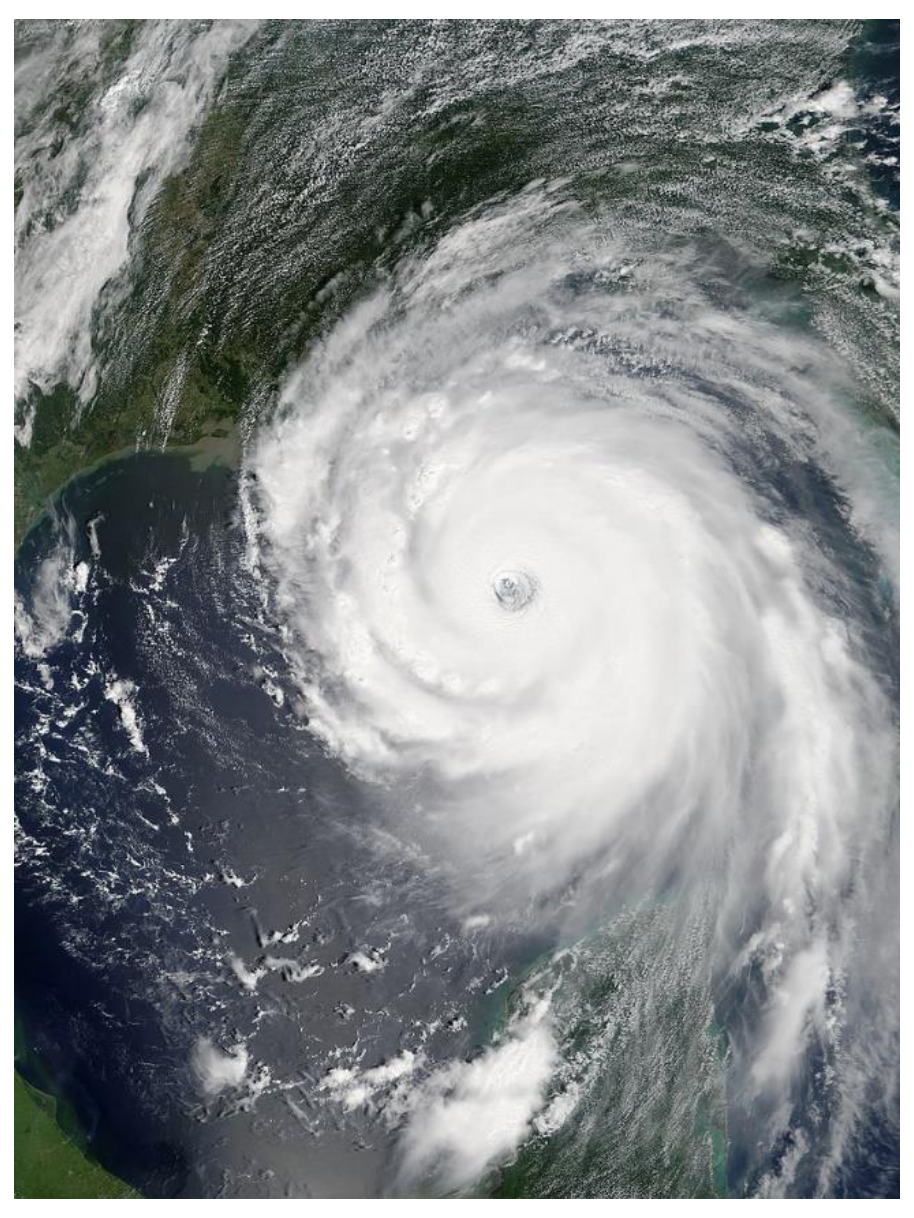
Tropical cyclones are one of the most concerning atmospheric phenomena, especially in the light of climate change. Depending on the region, they are better known as hurricanes, typhoons etc. In Maps3 folder, you can find a map on which a hurricane is present. The center of rotation in the storm is known as "eye". The purpose of this task is to analyze the relevance of geostrophic approximation in studying tropical cyclones and, if needed, replace it with a more suitable one.
The latitude of the hurricane is . In order to measure the radius of the hurricane, we will use an approximation. Calibrate the ruler in Tracker with the width (distance from the leftmost to the rightmost point) of Hispaniola Island (the island on which the Dominican Republic and Point-du-Prince are situated), which is known to be of approximate 650 km.
B9 Estimate the Rossby number for the hurricane, taking for velocity scale the velocity depicted in the image and for distance scale the distance from the pinned point to the eye of the hurricane. [1 т.]
B10 Compare the Rossby number for the hurricane to the numbers obtained in B6 and comment about the validity of geostrophic approximation. If necessary, use the definition of Rossby number and the balance of forces to obtain a better approximation for flows at high enough altitude to disregard friction with the terrestrial surface. [1 т.]
The maps used in Part B are obtained from Windy.com.
Experimental task designed by
Tudor-Gabriel MOCIOI, Ecole Polytechnique, Paris
Andrei MARIN, University of Bucharest
Appendix 1
Given a set of points , that supposedly fit on a circle, we would like to find the radius of this circle. We suggest two possible methods.
Method 1 – Geometrical approach
Given three points in the plane, we can construct a circle containing all three points in the following way:
- Select a pair of points out of the set of three. Construct the perpendicular bisector of the segment determined by the two points.
- Select another pair of points out of the three. Construct its perpendicular bisector.
- Find the intersection of these perpendicular bisectors. This point will be exactly the center of the circle.
- Finally, construct the circle with the found center, going through any of the three points.
Clearly, the radius of this circle will be given by the distance between the center and one of the points on the circle.
To use this method, you might find the following assertion useful: the product of the slopes of two perpendicular lines is equal to .
Method 2 – Calculus-based
Given a curve in the plane, its curvature radius at a particular point is given by
For a curve described by a discrete set of points , we can approximate the first and second derivatives numerically.
Решение
Внимание: Непълно решение
В архива няма официално решение на тази задача.
Оригинал в Архива: exp.pdf