Съдържание

BAAO 2021, Теория — Задача 1. Mercury’s Rotation Period with Aricebo

Оригинал на условието (PDF)Съобщи за грешка

Всички материали от BAAO 2021

British Astronomy and Astrophysics Olympiad 2020-2021 — Astronomy & Astrophysics Competition Paper — Saturday 27th February 2021 · 27 февруари 2021 г. · 25 т.

Указания

Time: 3 hours ( $\sim 45$ minutes for Q1, $\sim 65$ minutes for Q2 and $\sim 70$ minutes for Q3).

Questions: All three questions should be attempted. Each question contains independent parts so that later parts can be attempted even if earlier parts are incomplete.

Solutions: Answers and calculations are to be written on loose paper ON ONE SIDE ONLY. Students should ensure their name and school is clearly written on the first answer sheet and that all pages are numbered. EACH QUESTION ANSWERED must be started on a new page. A standard formula booklet with standard physical constants may be used if desired.

Instructions: This paper will be invigilated over Zoom with all candidates starting at 9am, however please do not discuss any aspect of the paper on the internet until 9am Saturday 6 $^{\mathrm{th}}$ March.

Clarity: Solutions must be written legibly, in black pen (the papers are scanned), and working down the page. Scribble will not be marked and overall clarity is an important aspect of this exam.

Eligibility: The International Olympiad will be held during November 2021; all sixth form students are eligible to participate.

Calculators: Any standard calculator may be used, but calculators cannot be programmable and must not have symbolic algebra capability.

Training Dates and the IOAA (Bogota, Colombia, November 2021)

The team will be selected from Y12 students taking this paper as well as Y12 students taking the Senior Physics Challenge paper in March. The best students that are eligible to represent the UK at the IOAA will be invited to attend the Training Camp to be held online from (Tuesday 6 $^{\mathrm{th}}$ April to Saturday 10 $^{\mathrm{th}}$ April 2021). Astronomy material will be covered; problem solving skills and observational skills (telescope and naked eye observations) will be developed. At the Training Camp a Data Analysis exam along with a Round 3 theory paper will be sat. A team of five students (plus one reserve) will be selected for further training, mostly done remotely with (hopefully) additional training camps in the summer.

Important Constants

Constant	Symbol	Value
Speed of light	$c$	$3.00\times10^{8}\ \mathrm{m\,s^{-1}}$
Earth’s rotation period	1 day	24 hours
Earth’s orbital period	1 year	365.25 days
parsec	pc	$3.09\times10^{16}\ \mathrm{m}$
Astronomical Unit	au	$1.50\times10^{11}\ \mathrm{m}$
Radius of the Sun	$R_{\odot}$	$6.96\times10^{8}\ \mathrm{m}$
Radius of the Earth	$R_{\oplus}$	$6.37\times10^{6}\ \mathrm{m}$
Mass of the Sun	$M_{\odot}$	$1.99\times10^{30}\ \mathrm{kg}$
Mass of the Earth	$M_{\oplus}$	$5.97\times10^{24}\ \mathrm{kg}$
Luminosity of the Sun	$L_{\odot}$	$3.85\times10^{26}\ \mathrm{W}$
Stephan-Boltzmann constant	$\sigma$	$5.67\times10^{-8}\ \mathrm{J\,m^{-2}\,K^{-4}}$
Gravitational constant	$G$	$6.67\times10^{-11}\ \mathrm{m^{3}\,kg^{-1}\,s^{-2}}$
Boltzmann constant	$k_{\mathrm{B}}$	$1.38\times10^{-23}\ \mathrm{J\,K^{-1}}$
Permittivity of free space	$\varepsilon_0$	$8.85\times10^{-12}\ \mathrm{F\,m^{-1}}$
Permeability of free space	$\mu_0$	$4\pi\times10^{-7}\ \mathrm{H\,m^{-1}}$
Planck’s constant	$h$	$6.63\times10^{-34}\ \mathrm{J\,s}$
Elementary charge	$e$	$1.60\times10^{-19}\ \mathrm{C}$
Proton rest mass	$m_{\mathrm{p}}$	$1.67\times10^{-27}\ \mathrm{kg}$
Electron rest mass	$m_{\mathrm{e}}$	$9.11\times10^{-31}\ \mathrm{kg}$
Wien’s displacement law	$\lambda_{\max}T$	$2.90\times10^{-3}\ \mathrm{m\,K}$
Avagadro’s constant	$N_A$	$6.02\times10^{23}\ \mathrm{mol^{-1}}$

Basic calculus formulae:

Chain rule

\frac{\mathrm{d}}{\mathrm{d}x}f(g(x)) = f'(g(x))g'(x)

Product rule

\frac{\mathrm{d}}{\mathrm{d}x}(uv) = \frac{\mathrm{d}u}{\mathrm{d}x}v + u\frac{\mathrm{d}v}{\mathrm{d}x}

Quotient rule

\frac{\mathrm{d}}{\mathrm{d}x}\left(\frac{u}{v}\right) = \frac{\frac{\mathrm{d}u}{\mathrm{d}x}v - u\frac{\mathrm{d}v}{\mathrm{d}x}}{v^2}

Integration by parts

\int u\frac{\mathrm{d}v}{\mathrm{d}x}\,\mathrm{d}x = uv - \int v\frac{\mathrm{d}u}{\mathrm{d}x}\,\mathrm{d}x

Standard integral

\int\frac{1}{x}\,\mathrm{d}x = \ln|x| + C

Important Formulae

You might find the diagram of an elliptical orbit below useful in solving some of the questions:

Elements of an elliptic orbit:

$a = \mathbf{OA}\ (= \mathbf{OP})$	semi-major axis
$b = \mathbf{OB}\ (= \mathbf{OC})$	semi-minor axis
$e = \sqrt{1 - \frac{b^2}{a^2}}$	eccentricity
$\mathbf{F}$	focus
$\mathbf{PF} = a(1-e)$	periapsis distance (shortest distance from $\mathbf{F}$ )
$\mathbf{AF} = a(1+e)$	apoapsis distance (longest distance from $\mathbf{F}$ )

Kepler’s Third Law: For an elliptical orbit, the square of the period, $T$ , of an object about the focus is proportional to the cube of the semi-major axis, $a$ (as defined above), such that

T^2 = \frac{4\pi^2}{GM}a^3\ ,

where $M$ is the total mass of the system (typically dominated by the central object) and $G$ is the universal gravitational constant.

Vis-Viva Equation: For an elliptical orbit, the speed $v$ of an object at a distance $r$ from the focus is related to the semi-major axis, $a$ , total mass of the system, $M$ , and universal gravitational constant, $G$ , (as defined above), such that

v^2 = GM\left(\frac{2}{r} - \frac{1}{a}\right)\ .

Magnitudes: The apparent magnitudes of two objects, $m_1$ and $m_0$ , are related to their apparent brightnesses, $b_1$ and $b_0$ , via the formula

\frac{b_1}{b_0} = 10^{-0.4(m_1 - m_0)}\ .

The absolute magnitude of an object, $\mathcal{M}$ , is the same as its apparent magnitude when viewed from 10 pc, hence the relationship between apparent and absolute magnitude and distance is

m - \mathcal{M} = 5\log\left(\frac{d}{10}\right)\ ,

where $d$ is measured in parsecs.

BAAO 2020/21 Solutions and Marking Guidelines

Note for markers:

Answers to two or three significant figures are generally acceptable. The solution may give more in order to make the calculation clear. Units should be present on final answers when appropriate.
There are multiple ways to solve some of the questions; please accept all good solutions that arrive at the correct answer. Students getting the answer in a $\boxed{\text{box}}$ will get all the marks available for that calculation / part of the question (as indicated in red), so long as there are no unphysical / nonsensical steps or assumptions made (students may not explicitly calculate the intermediate stages and should not be penalised for this so long as their argument is clear).

Условие

In November 2020 the Aricebo Telescope at the National Astronomy and Ionosphere Centre (NAIC) in Puerto Rico was decommissioned due to safety concerns after extensive storm damage. First opened in November 1963, this brought an end to an illustrious contribution to radio astronomy where, with a dish diameter of 304.8 m (1000 ft), it was the largest radio telescope in the world until 2016. Its important discoveries range from detection of the first extrasolar planets around a pulsar to fast radio bursts, as well as a pivotal role in the search for extraterrestrial intelligence (SETI), however in this question we will explore its earliest major revelation: that Mercury was not tidally locked.

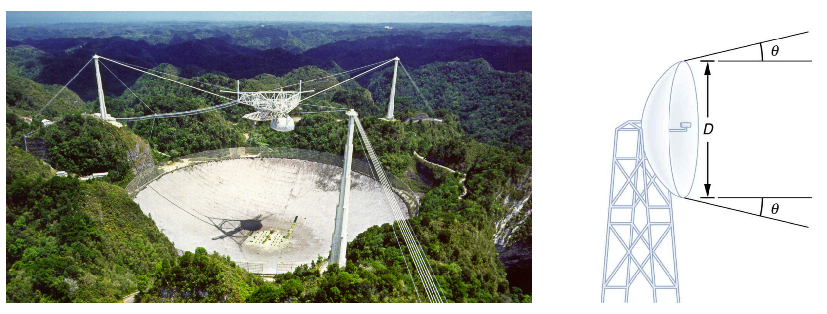
Left: aerial photograph of the Arecibo radio dish in a forested valley with its suspended receiver platform and support towers. Right: line drawing of a dish antenna of diameter D on a lattice tower, with the transmitted beam edges diverging from the dish rim by angle θ at top and bottom. — Figure 1: *Left*: The Aricebo telescope before it was damaged. Credit: NAIC. *Right*: When transmitting a pulse from a radio telescope, diffraction prevents the beam from staying perfectly parallel and so the width of the beam increases by $2\theta$ . Credit: OpenStax, College Physics.

Mercury had already been studied with optical and infrared telescopes, however the advantage of a radio telescope was that you could send pulses and receive their reflections. This radar-ranging technique had already been used with Venus to measure the distance to it and hence provide the data necessary for a definitive measurement of an astronomical unit in metres.

The radar echo from Mercury is much harder to detect due to the extra distance travelled and its smaller cross-sectional area (its radius is $2440$ km). In April 1965, Pettengill and Dyce sent a series of $500$ µs pulses at $430$ MHz with a transmitted power of $2.0$ MW towards Mercury whilst it was at its closest point in its orbit to Earth. In ideal circumstances the beam would stay parallel, however diffraction widens the beam as shown on the right in Fig 1.

a. Calculate the power of each echo received by the Aricebo telescope and hence determine the total number of photons in each echo, given the echo was detected $579.3$ s after being transmitted and Mercury’s surface only reflects $6.5\%$ of the incident radio photons. Assume $\theta = 0.16^{\circ}$ and the reflected photons from Mercury are scattered randomly within only the hemisphere facing Earth. [8 т.]

The signal-to-noise ratio of this echo was high enough that Doppler broadening of the received signal was reliably detected, allowing a determination of the rotation rate of Mercury. In August 1965 the same scientists sent $100$ µs pulses and sampled the echo on short timescales as it returned. The strongest echo (received first) came from the point of the planet closest to the Earth (called the sub-radar point), with later echos coming from other parts of the surface in an annulus of increasing radius (see Fig 2).

Photons from the approaching side would be blueshifted to a higher frequency, whilst those from the receding side would be redshifted to a lower frequency. Hence, by measuring the Doppler shift and the time delay, you can map the rotational velocity as a function of apparent longitude and so can calculate the apparent rotation rate (as well as the direction of rotation and co-ordinates of the pole).

Left: six stacked echo spectra labelled by relative delay (−60 µs, 0, 120 µs, 210 µs, 300 µs, 390 µs) with scale factors (3, 8, 3, 1, 1, 1), 'ASSUMED CENTER' arrow at top, small arrows marking the two Doppler-shifted peaks, horizontal axis 'RELATIVE FREQUENCY (c/s)' from 0 to 8.0. Top right: disc of the planet with the projection of the apparent rotation axis (ω), apparent equator, approaching and receding edges, an annulus defined by time delay and two vertical strips defined by Doppler shift. Bottom right: 'MERCURY SPECTRUM 17 AUG. 1965', echo power (0 to 1.0) versus frequency (c/s) from −3 to 4, peaked at 0. — Figure 2: *Left*: Snapshots of the reflections of a single $100$ µs pulse. The strength of the echo weakens as you move to later delays (as represented by the scale factor in the top right of each snapshot) and hence you need to use an annulus rather than detections from the horizon. The small arrows indicate the Doppler shifted frequency associated with intersection of the annulus with the apparent equator for each delay. The horizontal axis is in cycles per second (and so 1 c/s = 1 Hz). Credit: Dyce, Pettengill and Shapiro (1967). *Top right*: The key principles of the delay-Doppler technique, looking at a cross-section of the planet. At the very centre is the sub-radar point (the point on the planet’s surface closest to the Earth). As you move away from the sub-radar point the light has to travel further before it can be reflected, and hence the echo from those regions arrives later. The brightest point of any given annulus is where it intersects the apparent equator (due to the largest reflecting area), and so in each of the snapshots that is why the extreme Doppler shifts are boosted relative to the middle. Credit: Shapiro (1967). *Bottom right*: The same as the snapshots, but this time summed over the first $500$ µs of reflections. Here the difference between the extreme left and right frequencies reliably detected is $\sim 5$ Hz, but when corrected for relative motion of the Earth and Mercury it becomes the value given in part c. Credit: Pettengill, Dyce and Campbell (1967).

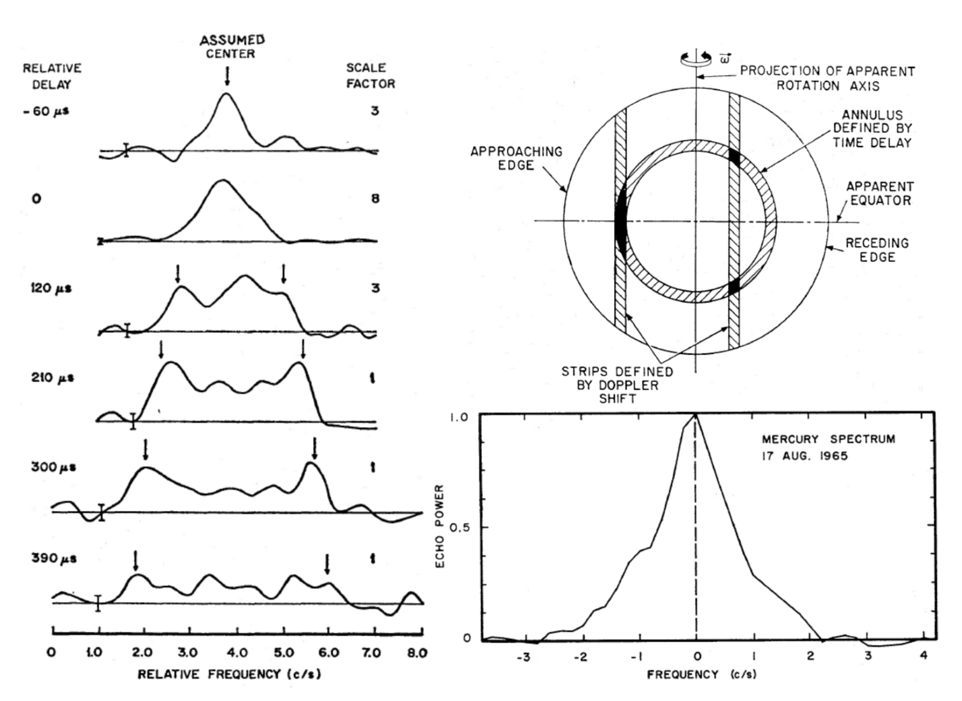
The Doppler shift with light is given as

\frac{\Delta f}{f} = \frac{v}{c}\ ,

where $\Delta f$ is the shift in frequency $f$ , $v$ is the line-of-sight velocity of the emitting object and $c$ is the speed of light.

b. (i) Averaging over a series of pulses from August 1965, after correcting for the relative motion of the Earth and Mercury and the rotation rate of the Earth during the observations, the difference between the frequencies of photons from the extreme left and right parts of an annulus received $500$ µs after the initial echo was $\Delta f_{\mathrm{total}} = 4.27$ Hz.

Given that the pulse was Doppler shifted twice (once when reflected, once again when received back at Aricebo) show that the rotational period of Mercury is $\sim 60$ days. Assume that the axis of rotation is normal to the plane of observations. [1 day = 24 hours] [6 т.]

b. (ii) Mercury has a semi-major axis of $0.387$ au. Rounding slightly if necessary, express the ratio orbital period : rotational period in a simple integer form (the integers should be $< 10$ ). [3 т.]

Ever since the first maps of Mercury’s surface by Schiaparelli in the late 1880s, many in the scientific community believed that Mercury would be tidally locked and so always present the same hemisphere to the Sun. The reason they expected the rotational period to be the same as its orbital period (i.e. a $1:1$ ratio), rather like the Moon, is because it is so close to the Sun and the tidal torques causing this synchronicity are proportional to $r^{-6}$ where $r$ is the distance from the massive body. Given it is the closest planet to the Sun, it receives by far the largest torques, so the discovery it was in a different ratio was a complete surprise to many of the scientists at the time.

c. (i) The eccentricity of the planet’s orbit became the prime suspect as to why its actual ratio would be stable over long time periods.

Calculate how many times larger the tidal torque is when Mercury is at perihelion than when it is at aphelion, given the eccentricity of the orbit is 0.206. [1 т.]

c. (ii) Assuming the tidal torque at perihelion is the dominating factor in setting Mercury’s rotation rate, predict the rotational period of Mercury if it were to behave as though it was tidally locked when passing through perihelion. Compare this to the measured value and comment on validity of the assumption. [5 т.]

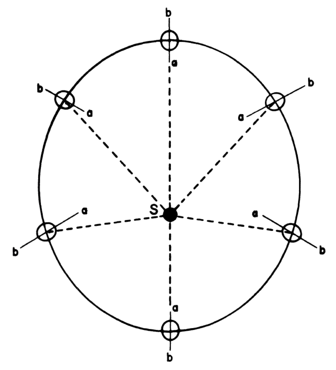
c. (iii) Fig 3 shows the orientation of Mercury’s axis of minimum moment of inertia (the axis the tidal torque acts upon) if the ratio had been $1:1$ . Redraw this diagram but for the ratio found in part b (ii). Assume the initial orientation at perihelion looks the same in both cases (so only the other five positions are needed, separated equally in time) and that the planet both orbits and rotates in an anticlockwise direction. [Note: the orientation when it returns to perihelion may not be the same as it was initially.] [2 т.]

Elliptical orbit with the Sun S (filled dot) near the centre and dashed lines to six positions of Mercury (circles with crosses); at each position the axis is drawn with ends labelled a (towards the Sun) and b (away from the Sun), the axis always pointing along the Sun–planet line. — Figure 3: The orientation of Mercury’s axis of minimum moment of inertia (the axis the tidal torque acts upon) displayed at six points in its orbit (equally spaced in time) if the ratio had been $1:1$ . Credit: Colombo and Shapiro (1966).

Отговори

Решение

Q1 – Mercury Rotation Period with Aricebo [25 marks]

a. We can use the light travel time to get the distance to Mercury

d_{Merc} = c \times \frac{t_{Merc}}{2} = 3.00\times10^{8}\times\frac{579.3}{2} = 8.69\times10^{10}\ \mathrm{m} \qquad [1]

From this we can work out the radius of the beam

r_{beam} = d_{Merc}\tan\theta = 8.69\times10^{10}\times\tan 0.16^{\circ} = 2.43\times10^{8}\ \mathrm{m} \qquad [1]

[Accept $r_{beam} = d_{Merc}\tan\theta + R_{Aricebo}$ although the effect of $R_{Aricebo}$ is negligible as Mercury is so far away. Also accept small angle approximation if $\theta$ is correctly converted into radians]

Consequently the intensity of the beam at Mercury is then

b_{Merc} = \frac{P}{\pi r_{beam}^2} = \frac{2.0\times10^{6}}{\pi(2.43\times10^{8})^2} = 1.08\times10^{-11}\ \mathrm{W\,m^{-2}} \qquad [1]

This means the total power reflected is

P_{refl} = b_{Merc}\times\pi R_{Merc}^2\times0.065 = 1.08\times10^{-11}\times\pi(2440\times10^{3})^2\times0.065 = 13.1\ \mathrm{W} \qquad [1]

Treating it as a point source radiating in just the hemisphere that faces Earth

b_{Earth} = \frac{P_{refl}}{2\pi d_{Merc}^2} = \frac{13.1}{2\pi(8.69\times10^{10})^2} = 2.77\times10^{-22}\ \mathrm{W\,m^{-2}} \qquad [1]

Consequently, the power received by Aricebo is

P_{received} = b_{Earth}\times\pi R_{Aricebo}^2 = 2.77\times10^{-22}\times\pi\left(\frac{304.8}{2}\right)^2 = \boxed{2.02\times10^{-17}\ \mathrm{W}} \qquad [1] \quad \mathbf{[6]}

Turning this into a number of photons:

E_{phot} = hf = 6.63\times10^{-34}\times430\times10^{6} = 2.85\times10^{-25}\ \mathrm{J} \qquad [1]

n = \frac{E_{tot}}{E_{phot}} = \frac{P_{recieved}t_{pulse}}{E_{phot}} = \frac{2.02\times10^{-17}\times500\times10^{-6}}{2.85\times10^{-25}} = \boxed{35500\ \mathrm{photons}} \qquad [1] \quad \mathbf{[2]}

[This drop in power of $10^{23}$ is why you need such a powerful transmitter and such a large receiving dish to pick up the echo, and hence why it was such a hard measurement to make at the time]

b. i.

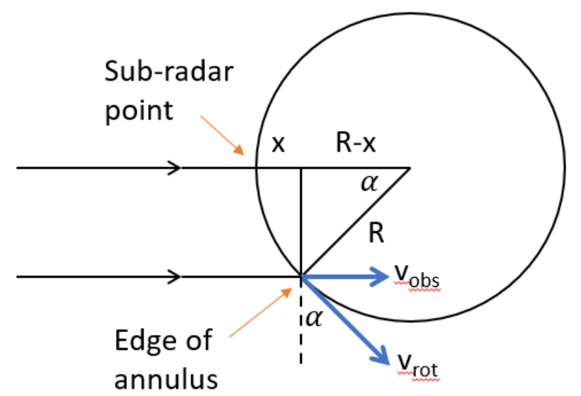
Cross-section of Mercury as a circle of radius R with two incoming horizontal beams; the upper one reaches the sub-radar point, the lower one the edge of the annulus at depth x (R-x marked along the axis, angle α at the centre); at the edge point the rotational velocity v_rot is drawn tangentially and its line-of-sight component v_obs horizontally, with angle α between v_rot and the vertical dashed line.

Helpful diagram of the situation [1]

Calculating x from the path difference between a beam that reflects of the sub-radar point and the edge of the annulus:

x = c\times\frac{1}{2}t = 3.00\times10^{8}\times\frac{1}{2}\times500\times10^{-6} = 7.50\times10^{4}\ \mathrm{m} \qquad [1]

We can now calculate α,

\cos\alpha = \frac{R-x}{R} = \frac{2440-75}{2440} = 0.969 \therefore \alpha = 14.2^{\circ} \qquad [1]

Using the Doppler effect equation given, with $\Delta f$ halved twice (once for the two journeys, once to compare from sub-radar point to edge rather than edge to edge),

v_{obs} = \frac{\frac{1}{4}\Delta f_{total}}{f}c = \frac{\frac{1}{4}\times4.27}{430\times10^{6}}\times3.00\times10^{8} = 0.745\ \mathrm{m\,s^{-1}} \qquad [1]

Considering the geometry of the situation to get the tangential (rotational) velocity,

v_{rot} = \frac{v_{obs}}{\sin\alpha} = \frac{0.745}{\sin 14.2^{\circ}} = 3.027\ \mathrm{m\,s^{-1}} \qquad [1]

\therefore T_{rot} = \frac{2\pi R_{Merc}}{v_{rot}} = \frac{2\pi\times2440\times10^{3}}{3.027} = 5.06\times10^{6}\ s = \boxed{58.6\ \mathrm{days}} \qquad [1] \quad \mathbf{[6]}

[Students using $v_{rot} = \frac{\Delta f_{total}}{f}c = 2.98\ m\ s^{-1}$ to get $T_{rot} = 59.56$ days only get the final mark for ecf on their v $_{\mathrm{rot}}$ (i.e. 1 out of 6). T $_{\mathrm{rot}}$ can be given in seconds or days, but if in the former a comparison to 60 days must be made]

[We are fortunate that the rotational axis of mercury is almost perfectly normal to the plane of observations, so this is almost identical to the real rotational period]

ii. From Kepler’s third law,

T_{orb} = \sqrt{\frac{4\pi^2a^3}{GM_{\odot}}} = \sqrt{\frac{4\pi^2}{6.67\times10^{-11}\times1.99\times10^{30}}\times(0.387\times1.50\times10^{11})^3} = 7.63\times10^{6}\ \mathrm{s} = 88.28\ \mathrm{days} \qquad [1]\,[1]

We can now work out the ratio

\therefore \text{ratio} = \frac{T_{orb}}{T_{rot}} = \frac{88.2836}{58.617} = 1.506 \approx 1.5 \qquad \text{[allow ecf with } T_{rot} = 60 \text{ days]} \qquad [0.5]

\therefore \boxed{3:2} \qquad [0.5] \quad \mathbf{[3]}

c. i. Given $r_{peri} = a(1-e)$ and $r_{aph} = a(1+e)$ and $\tau \propto r^{-6}$

\therefore \frac{\tau_{peri}}{\tau_{aph}} = \left(\frac{r_{peri}}{r_{aph}}\right)^{-6} = \left(\frac{1-e}{1+e}\right)^{-6} = \left(\frac{1-0.206}{1+0.206}\right)^{-6} = \boxed{12.3} \qquad [1] \quad \mathbf{[1]}

ii. Finding the perihelion distance first

r_{peri} = a(1-e) = (0.387\times1.50\times10^{11})(1-0.206) = 4.61\times10^{10}\ \mathrm{m} \qquad [1]

[Give this mark if they have already calculated r $_{\mathrm{peri}}$ in c) i) instead]

Using the vis-viva equation given at the beginning of the paper,

v_{peri} = \sqrt{GM_{\odot}\left(\frac{2}{r_{peri}} - \frac{1}{a}\right)} = \sqrt{6.67\times10^{-11}\times1.99\times10^{30}\left(\frac{2}{4.61\times10^{10}} - \frac{1}{0.387\times1.50\times10^{11}}\right)} = 5.89\times10^{4}\ \mathrm{m\,s^{-1}} \qquad [1]

Working out the orbital angular velocity,

\omega_{orb} = \frac{v_{peri}}{r_{peri}} = \frac{5.89\times10^{4}}{4.61\times10^{10}} = 1.28\times10^{-6}\ \mathrm{rad\,s^{-1}} \qquad [1]

If $\omega_{orb} = \omega_{rot}$ [which gives $v_{rot} = 3.12\ \mathrm{m\,s^{-1}}$ ]

\therefore T_{rot} = \frac{2\pi}{\omega_{rot}} = \frac{2\pi}{1.28\times10^{-6}} = 4.91\times10^{6}\ \mathrm{s} = \boxed{56.9\ \mathrm{days}} \qquad [1] \quad \mathbf{[4]}

This is similar to the measured value of T $_{\mathrm{rot}}$ ∴ valid assumption [1] [1]

iii.

New axes are alternating vertical and horizontal lines [1] [1]

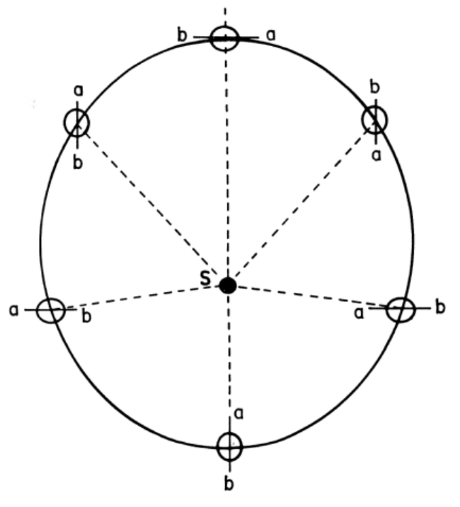
Redrawn Figure 3 for the 3:2 resonance: elliptical orbit with the Sun S and six equally spaced positions; the axis a–b alternates between horizontal and vertical at successive positions, with ends a and b labelled.

Ends for a & b correctly labelled [1] [1]

[This does mean that it needs two Mercurian years before the perihelion orientation is the same – as such one (solar) day on Mercury lasts two years!]

END OF PAPER

Questions proposed by:
Dr Alex Calverley (Royal Grammar School, Guildford)
Niam Vaishnav (University of Oxford)
Nick Koukoufilippas (University of Oxford)

Оригинал в Архива: BAAO_2021.pdf · официални решения: BAAO_2021_solutions.pdf