Балкански 2024, Теория — Задача 3. Wind at the national weather forecast scale

1. Atmospheric equilibrium models

We consider air in equilibrium in the terrestrial reference frame $R$. Each element of this fluid is therefore in equilibrium under the action of forces external to this element, which are of two types: pressure forces and the force due to the gravitational field.

1. Air being an ideal gas, calculate its density $\rho_0 = \rho(P_0, T_0)$ under normal conditions - temperature $T_0 = 273K$ and pressure $P = P_0$.

2. We choose an orthonormal reference system in $R$. The state of the atmosphere is characterized by the pressure fields $P(x, y, z)$ and temperature fields $T(x, y, z)$:

2. (a) Write the mechanical equilibrium condition of air subjected to pressure forces and the gravity field, assumed to be locally uniform.

2. (b) Deduce that P only depends on $z$ and establish the equation allowing us to determine $P(z)$ as a function of $M_a, P, g, T$ and the ideal gas constant $R$.

3. We first consider the atmosphere in isothermal equilibrium.

3. (a) Justify that the pressure varies with the altitude $z$ according to a law of the type

where $H$ is a length called the scale height of the atmosphere to be expressed as a function of $M_a, R, g$ and $T$. Calculate the scale height $H_0$ of the isothermal atmosphere at $T_0 = 273K$.

3. (b) Is the assumption of uniform temperature justified?

4. We now consider the atmosphere in adiabatic equilibrium characterized at any altitude by the relation $P = K\rho^{\gamma}$ where $K$ is a constant and $\gamma = \frac{C_p}{C_v} \approx 1.4$ is the ratio of the heat capacities at constant pressure and volume of ideal diatomic gases.

4. (a) Discuss how we can find the explicit form of $P(z)$ and $T(z)$. From now on we assume that their explicit forms are:

4. (b) Numerically calculate the vertical temperature gradient in $Kkm^{-1}$ corresponding to this model of atmosphere in adiabatic equilibrium.

4. (c) Trace the general appearances of the pressure variations and its gradient as a function of altitude. (The general appearance is requested and not the precise one!)

4. (d) Numerically calculate the pressure gradient for $z = 0, 2500$ and $5000m$.

4. (e) From the pressure gradients found, give an order of magnitude of the scale of the vertical dimension $L_z$ on which the pressure varies by $100Pa$.

4. (f) Express the ratio of the air densities $\rho(P, T)/\rho(P_0, T_0)$ as a function of $z, H_0$ and $\gamma$. Calculate $\rho$ at $2500m$ altitude.

2. Dynamics of atmospheric movements: the geostrophic wind

5. Figure 4 shows the isobaric lines in $hPa$ and separated by $2hPa$ each, at sea level in Western Europe on 23 January 2002 at midnight.

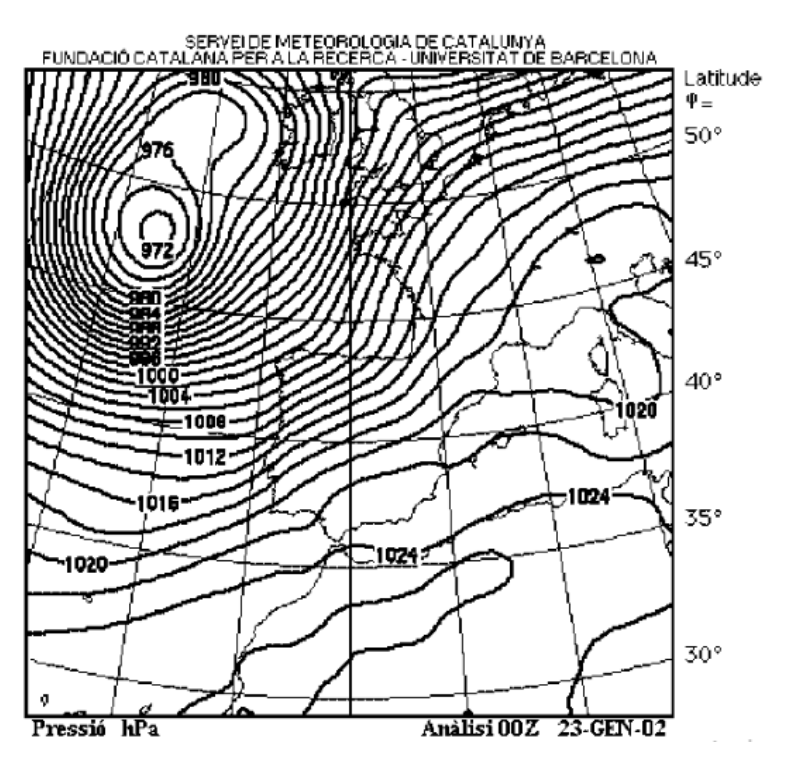
5. (a) Determine on this pressure map the value of the horizontal pressure gradient in Bordeaux. Compare with the data in Table 1. From now on, the value of the horizontal pressure gradient used in numerical applications will be that given by Table 1.

5. (b) Knowing that we usually attribute horizontal dimensions $L_h$ to elementary domains such that the horizontal pressure varies on average by $100Pa$, determine an order of magnitude of $L_h$.

In the rest of the problem, we analyse on this scale.

6. (a) Give the expression of the Earth's gravitational field $\overrightarrow{g}^*(\overrightarrow{r})$ at a point identified by $\overrightarrow{r}$ relative to the center of the Earth, assumed to be a homogeneous sphere of mass $M_T$. We will denote by $G$ the universal gravitational constant.

6. (b) Propose an expression giving the variation with altitude $z$ of the module $g^*(z) = ||\overrightarrow{g}^*||$ as a function of the ratio $\frac{z}{r_T}$ and $g^*(0)$. What is the relative error committed at $2500m$ altitude if we replace $g^*(z)$ by $g_0^* = g^*(0)$.

7. Let $R_0$ be the terrestrial barycentric, geocentric reference frame, which we will consider as Galilean, and let $R_l$ be the local terrestrial reference frame, whose origin $O$ has latitude $\phi$ (Figure 5). We choose $Ox$ tangent to the parallel passing through $O$ and directed towards the East, $Oy$ tangent to the meridian passing through $O$ and directed towards the North. The reference frame $R_l$ is in motion with respect to $R_0$ by a uniform diurnal rotation movement of angular velocity $\omega$.

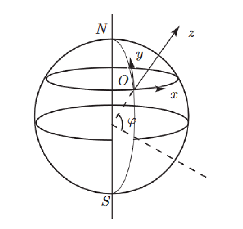
7. (a) Specify in $R_l$ the direction of the resulting acceleration $\overrightarrow{\Gamma}_E(\overrightarrow{r})$. For a point of altitude $z$ vertically above $O$, establish the expression of its modulus $\Gamma_E(z)$ as a function of $\omega, z, r_T$ and $\phi$. What is the relative error made on $\Gamma_E$ at $2500m$ altitude if we replace $\Gamma_E(z)$ by $\Gamma_{E0} = \Gamma_E(0)$. Calculate the typical value of $\Gamma_{E0}$ in France.

7. (b) Let $\overrightarrow{g}(\overrightarrow{r})$ be the local effective gravitational field, whose direction is given by that of a freely hanging pendulum. Deduce from the previous results the relationship between the gravitational field $\overrightarrow{g}(\overrightarrow{r})$, the terrestrial gravitational field $\overrightarrow{g}^*(\overrightarrow{r})$ and the resulting acceleration $\overrightarrow{\Gamma}_E(\overrightarrow{r})$. Justify the hypothesis of a locally uniform gravitational field $\overrightarrow{g}$ used in 1.

7. (c) A particle of mass $m$ moves at speed $\overrightarrow{V}$ in $R_l$. Give the expression for the inertial acceleration due to that speed $\overrightarrow{\Gamma_C}$ as a function of $\overrightarrow{V}$ and $\overrightarrow{\omega}$. Express this inertial force $\overrightarrow{F_C}$ in $Oxyz$ as a function of $m, \omega$, of latitude $\phi$ and of the components $(V_x, V_y, V_z)$ of $\overrightarrow{V}$.

8. The forces of gravity, inertia and pressure gradient act on moving atmospheric air. Write the vector equation of motion of a particle domain. Deduce the three equations giving the coordinates of the local acceleration $\overrightarrow{\Gamma} = \overrightarrow{A}$ in $Oxyz$.

9. We first propose to study the vertical movements of air within the framework of the adiabatic equilibrium atmosphere model.

9. (a) Evaluate the orders of magnitude of the different terms located in the second term of the equation of vertical motion, using the results found in question 4.d) when placed at an altitude of $2500m$, for a latitude of $\phi = 45^{\circ}$ and a wind of the order of $10ms^{-1}$. What can we deduce from this about the importance of the vertical component of the inertial force due to speed?

9. (b) Observations show that apart from very brief periods of adaptation to vertical disturbances, the updrafts or downdrafts are particularly stable over time. What can we conclude from this concerning the amplitude of the vertical acceleration? From the data in Table 1, estimate the order of magnitude of the vertical acceleration. By then making the legitimate simplifications, what does the equation of vertical air motion reduce to? Conclude with regard to the results of Part 1.

10. We now study the horizontal movements of the air by placing ourselves at an altitude of $2500m$.

10. (a) Based on the data in Table 1, simplify the equations of horizontal motion. We define the Coriolis parameter $k$ by $k = 2\omega sin\phi$: what are its respective numerical values at latitudes of $45^{\circ}$ in the Northern and Southern hemispheres.

10. (b) The horizontal relative velocity is defined by $\overrightarrow{V_h} = V_x\overrightarrow{e_x} + V_y\overrightarrow{e_y}$ . Show that the horizontal Coriolis force (the one carrying the parameter $k$) per unit mass can be expressed in the form: $f_{Ch} = -k(\overrightarrow{e_z} \wedge \overrightarrow{V_h})$. What can we conclude about the orientation of the vector $\overrightarrow{f_{Ch}}$ relative to the vector $\overrightarrow{V_h}$ in the Northern and Southern hemispheres?

10. (c) Calculate the modulus of the horizontal Coriolis force per unit mass $\overrightarrow{f_{Ch}}$ at an altitude of $2500m$ for which the wind has a horizontal speed of $15ms^{-1}$ at a latitude of $45^{\circ}$. Taking as the horizontal pressure gradient at the same altitude that given by Table 1, calculate the modulus of the horizontal pressure force per unit mass $\overrightarrow{f_{Ph}}$.

10. (d) In general, observations show that the tangential accelerations undergone by the particle domains in their horizontal movements are always very small in the large atmospheric movements in our mid-latitudes. Similarly, normal accelerations are generally very small except in front of moving depressions. Using the data in Table 1, estimate the order of magnitude of the moduli of the quantities $\overrightarrow{f_{Ch}}$, $\overrightarrow{f_{Ph}}$ and of the horizontal acceleration $\overrightarrow{\Gamma_h} = \overrightarrow{A_h}$. What can we conclude for the value of the vector sum $\overrightarrow{f_{Ph}} + \overrightarrow{f_{Ch}}$?

11. The fictitious wind with horizontal speed $\overrightarrow{V_g}$ which identically satisfies the equation $\overrightarrow{f_{Ph}} + \overrightarrow{f_{Ch}} = 0$ is called geostrophic wind.

11. (a) Show that this wind is entirely determined by knowledge of the spatial distribution of pressure and express its velocity field $\overrightarrow{V_g}$ using the horizontal pressure gradient $\overrightarrow{\nabla_h}(P)$.

11. (b) What is the value of the acceleration $\Gamma_g$ and the local nature of the trajectory of the particles constituting the geostrophic wind? Specify on a diagram the respective orientations of $\overrightarrow{V_g}$, $\overrightarrow{f_{Ph}}$ and $\overrightarrow{f_{Ch}}$ in the Northern and Southern hemispheres.

11. (c) Given the orders of magnitude in Table 1, verify that, for the latitude of $45^{\circ}$, the module $V_g$ of the geostrophic velocity is equal to $V_h$. Define using Figure 6 the latitude range for which the relative deviation $\frac{|V_g-V_h|}{V_h}$ remains less than $30\%$.

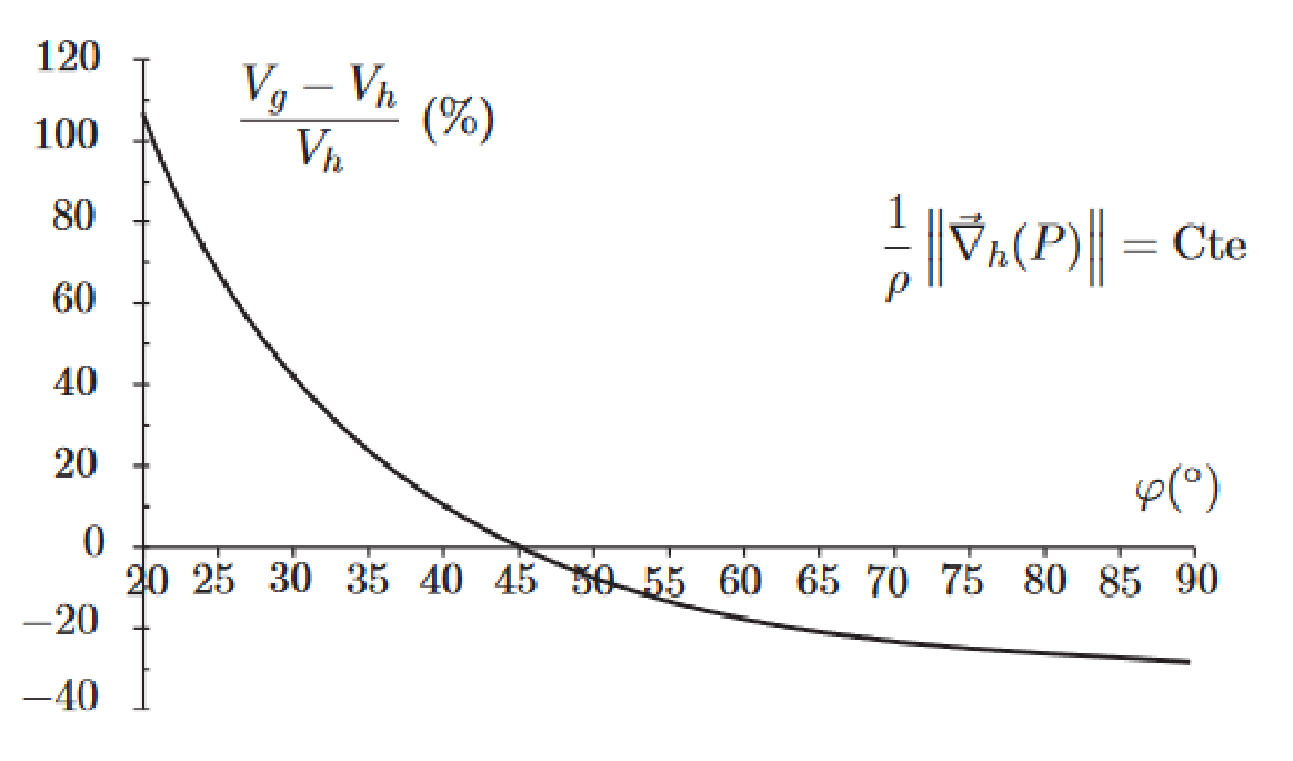
11. (d) Deduce the two conditions necessary for the geostrophic wind to be a good approximation $\overrightarrow{V_g} \approx \overrightarrow{V_h}$ of the real wind. Are these conditions verified at equatorial latitudes ($\phi < 20^{\circ}$)?