Балкански 2026, Теория — Задача 1. Phase-detection autofocus

I. Formation of a sharp image

1. State the Gaussian conditions and approximations under which the thin lens $(L)$ is used.

2. The object is represented by a segment $(AB)$ perpendicular to the optical axis and its image by $(A'B')$. The point $C$ is where the image sensor meets the axis. Define

Algebraic distances are positive from left to right, in the direction of light propagation; transverse segments are positive upwards and angles are positive counterclockwise.

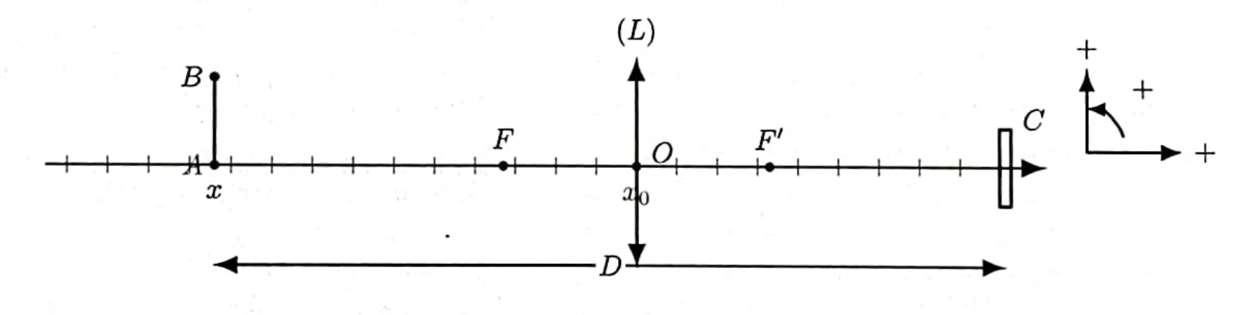
2. a) Starting from the Descartes thin-lens equation

derive the transverse magnification relation connecting $\overline{AB}$, $\overline{A'B'}$, $p$ and $p'$, and hence obtain Newton's conjugation relation connecting $\overline{FA}$, $\overline{F'A'}$ and $f'$.

2. b) On the copy of the figure provided on the supplementary sheet, construct $(A'B')$ with a ruler using two principal rays. Check the position of $A'$ using Newton's relation. Is the image formed on the sensor?

3. Let $D = |\overline{AC}|$ be the object-to-sensor distance and $T = \overline{OC} = -x_0 > 0$ the lens-to-sensor distance.

3. a) Assuming that the objective lies between the object and sensor, obtain the two possible solutions for $T$. Retain the solution $T < D/2$, corresponding to the objective close to the sensor, and show that

3. b) Find the condition on $D$ and $f'$ for these positions to be real. Give a geometrical interpretation of the limiting case.

3. c) Determine $T_\infty$ when the object is at infinity.

3. d) For $f' = 50\ \mathrm{mm}$, the objective must focus between infinity and $D_{\mathrm{min}} = 40\ \mathrm{cm}$. Calculate the required travel $\delta = T(D_{\mathrm{min}}) - T_\infty$. In which direction must the lens move as the object approaches?

3. e) A full-frame sensor of dimensions $36\ \mathrm{mm} \times 24\ \mathrm{mm}$ contains 24 million square pixels. The camera must resolve the $10\ \mathrm{cm}$ width of an object at $2.0\ \mathrm{km}$; require its image to span at least two pixels. Neglecting diffraction and aberrations, determine the minimum focal length. The numerical data in this part are independent of part d).

II. Study of the autofocus module

After unfolding the optical path, the system is represented below. The point $S$ is where the microlens plane meets the axis and $P$ is where the photosensor plane meets it.

When focus is correct, the intermediate image $(A'B')$ is formed in the plane of the field lens $(LC)$, whose optical centre is $O_c$. The microlenses lie in the image focal plane of $(LC)$, so $O_cS = f'_c$.

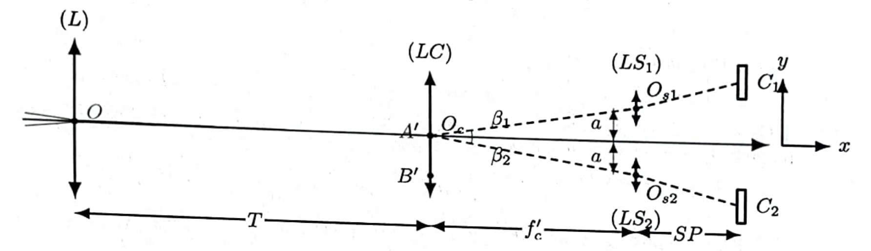
4. First consider the correctly focused configuration.

4. a) The plane containing $(LC)$ is conjugate to the photosensor plane through each microlens. Determine the distance $SP$.

4. b) On the corresponding figure on the supplementary sheet, complete the construction of the secondary images $(A''_1B''_1)$ and $(A''_2B''_2)$. The points $A''_1$ and $A''_2$, which are images of the axial point $A'$, lie at the respective centres of $(C_1)$ and $(C_2)$. Compare the orientation of the secondary images with that of $(A'B')$.

4. c) Explain the role of the field lens: why does it allow both microlenses to receive bundles from the same point of the intermediate image? Which measured quantity carries the defocus information?

4. d) For the axial point $A'$, use the geometry of the figure and the small-angle approximation to determine the two chief-ray angles $\beta_1$ and $\beta_2$ in terms of $a$ and $f'_c$. State their signs, then calculate their magnitude.

5. The objective remains fixed and the initially focused object moves by a small distance $\Delta x > 0$ towards the camera. The primary image point then moves by $\Delta x'$ beyond the sensor plane. Use $f' = 50\ \mathrm{mm}$ for numerical applications.

5. a) Starting from the thin-lens equation, show to first order that

For $D = 1.0\ \mathrm{m}$ and $\Delta x = 1.0\ \mathrm{cm}$, first calculate $\Delta x'$ using the exact value of $T$ obtained in Question 3a), then give the estimate obtained from $D \gg T$ and $T \simeq f'$.

5. b) $A'$, which lies to the right of $(LC)$, is a virtual object for that lens. If $A'_c$ is its image through $(LC)$, show that

Justify the approximation $\overline{O_cA'_c} \simeq \Delta x'$.

5. c) $\star$ Using the approximation from part b), let $s = f'_c - \Delta x'$ be the new object distance for the microlenses. Use their conjugation relation to show that both secondary images undergo the same longitudinal displacement

5. d) $\star$ Using the rays through the microlens centres, show to first order that

In the fixed photosensor plane, the centre of each profile follows the chief ray. Using the distance $SP$ found in Question 4a), show that

Calculate $\Delta x''_1$, $\Delta x''_2$, $\Delta y''_1$ and $\Delta y''_2$ numerically.

5. e) Describe the relative shift of the two intensity profiles on the sensors and calculate its value. Compare it with the photodiode pitch $d$. Briefly explain why correlation of the complete intensity profiles may nevertheless measure a shift smaller than one pitch. How does the sign of the shift distinguish focus in front of the sensor from focus behind it?

6. The objective is now moved so that the image is formed again on the sensor. The algebraic lens displacement $\Delta x_L$ is positive in the direction of light propagation.

6. a) What is the sign of $\Delta x_L$ when the object has approached, so that $\Delta x > 0$?

6. b) Linearising the thin-lens equation while the object and lens move simultaneously, show that

For $D = 1.0\ \mathrm{m}$ and $\Delta x = 1.0\ \mathrm{cm}$, first calculate $K_L$ and $\Delta x_L$ using the exact value of $T$, then give the estimate obtained from $D \gg T$ and $T \simeq f'$.

7. Describe a complete autofocus loop: acquisition of the two profiles, estimation of their relative shift, determination of the error sign, motor command, and stopping criterion. Also give one situation in which phase-detection autofocus performs poorly.