EuPhO 2022, Експеримент — Задача 1. E: Physics of illumination
EuPhO-2022 Experimental problems. Language: English · 20 т.
Условие
An incandescent light bulb produces light by heating a tungsten filament to a high enough temperature to emit black body radiation in the visible part of the spectrum, but a lot of energy is still wasted in the infrared part.
To quantify light as perceived by human vision, we use photometric units, which take into account sensitivity of the human eye to light of different wavelengths. The total amount of visible light emitted by a source into all directions is called luminous flux, measured in lumens . The amount of visible light received by a surface per unit of its area is called illuminance, in lux , and can be measured by a light meter.
When measuring quantities of light based solely on the energy it carries, we use radiometric units, which are expressed with conventional units of power. Radiometric counterpart of the luminous flux is radiant flux, measured in watts , and irradiance is the counterpart of the illuminance.
Today you will study thermal and illumination properties of light sources. The three tasks are mostly independent from each other. Sketch your setup for each task. No error analysis is required for Tasks 1 & 2.
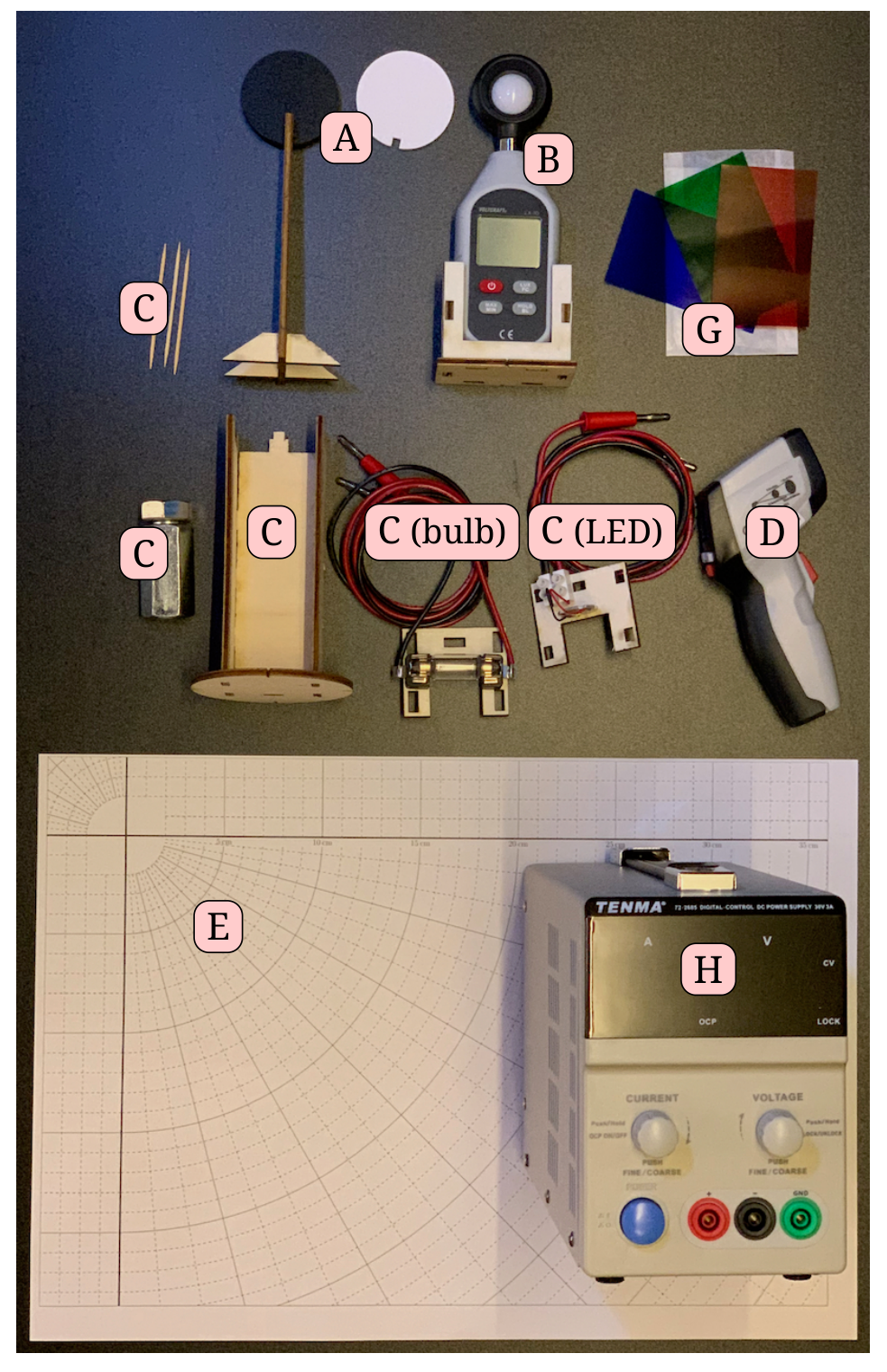
Equipment (see also Fig. 1)
A Black and white plastic plate thick with a stand. Both plates are good absorbers of infrared light.
B Light meter with a stand. The light meter turns off automatically after 6 minutes – turn it back on with a long press on the on/off button. Pay attention to the units (lx, not fc). You may use the HOLD button to freeze the displayed value.
C A light mounting stand with a round base, a weight for stability, and two interchangeable light modules: incandescent light bulb (maximum voltage ) and LED (maximum voltage , do not exceed current). You may use toothpicks to wedge the modules in place. Black paper is provided to shield your eyes while reading the instruments.
D Infrared thermometer. The measurement reading is held after a short delay when the trigger is released. The measurements may have a substantial but constant systematic error.
E Paper work mat with angular and distance grid.
F Protractor.
G Red, green and blue light filters in an envelope. If you have trouble telling the colours apart, raise the help card for assistance.
The filters are sensitive to heat. Keep them away from the light source.
H Power supply. Press the voltage/current knob multiple times to select which digit to adjust (indicated by the blinking light below the digit), and turn the knob to change the digit. After a few seconds, the light stops blinking and the display starts showing the actual voltage/current. Vary the current to control the light source. If the requested current cannot be reached without exceeding the maximum voltage, the power source will switch into the constant voltage mode and limit the current. Plug the wires into the matching negative (black) and positive (red) sockets of the power supply. Do not use the green socket.
To avoid damaging the light sources, set the voltage to allowed maximum and set the current to zero before you plug in the wires!
If your light source burns out, you can ask for a replacement. Note that only a limited number of spare light sources are available.
Task 1 - Colour and temperature (4 pts)
The colour of the black body radiation depends on its temperature. In astronomy, the temperature of stars is determined from their colour index, the ratio of illuminances measured through two different colour filters.
Task 1 (a) Table 1 contains the illuminances measured through the red, green and blue filter for a standard incandescent light source at known temperatures. Choose suitable light filters and construct a calibration curve that relates the chosen colour index to the temperature.
Task 1 (b) Measure the relationship between the electrical input power and the tungsten filament temperature. Plot the result over a relevant range.
Task 2 - Luminous efficacy (8 pts)
The performance of light sources is quantified by their luminous efficacy, measured in lumens per watt, as the ratio between the luminous flux and the consumed power. As a point of reference, the sun has luminous efficacy of .
Task 2 Measure the dependence of luminous efficacy on the electrical input power for both light sources across the range with detectable light output. Plot the results, one plot per light source. State all steps of the calculation procedure and present all the measured data. [8 т.]
Task 3 - Radiative heating (8 pts)
The following task may be time consuming, plan your work accordingly.
When light hits an object, some of it is absorbed. At moderate temperature differences between the object and the environment, we can model heat dissipation into the surroundings with the heat transfer coefficient , in the form , where is the temperature of the surface, the temperature of the surroundings, and denotes the power lost to the environment due to dissipation, per unit area.
Task 3 (a) Determine the heat transfer coefficient and the thermal conductivity for the black plastic, and perform error analysis. Assume the material absorbs all received light and the incandescent light bulb emits all power in the form of electromagnetic radiation.
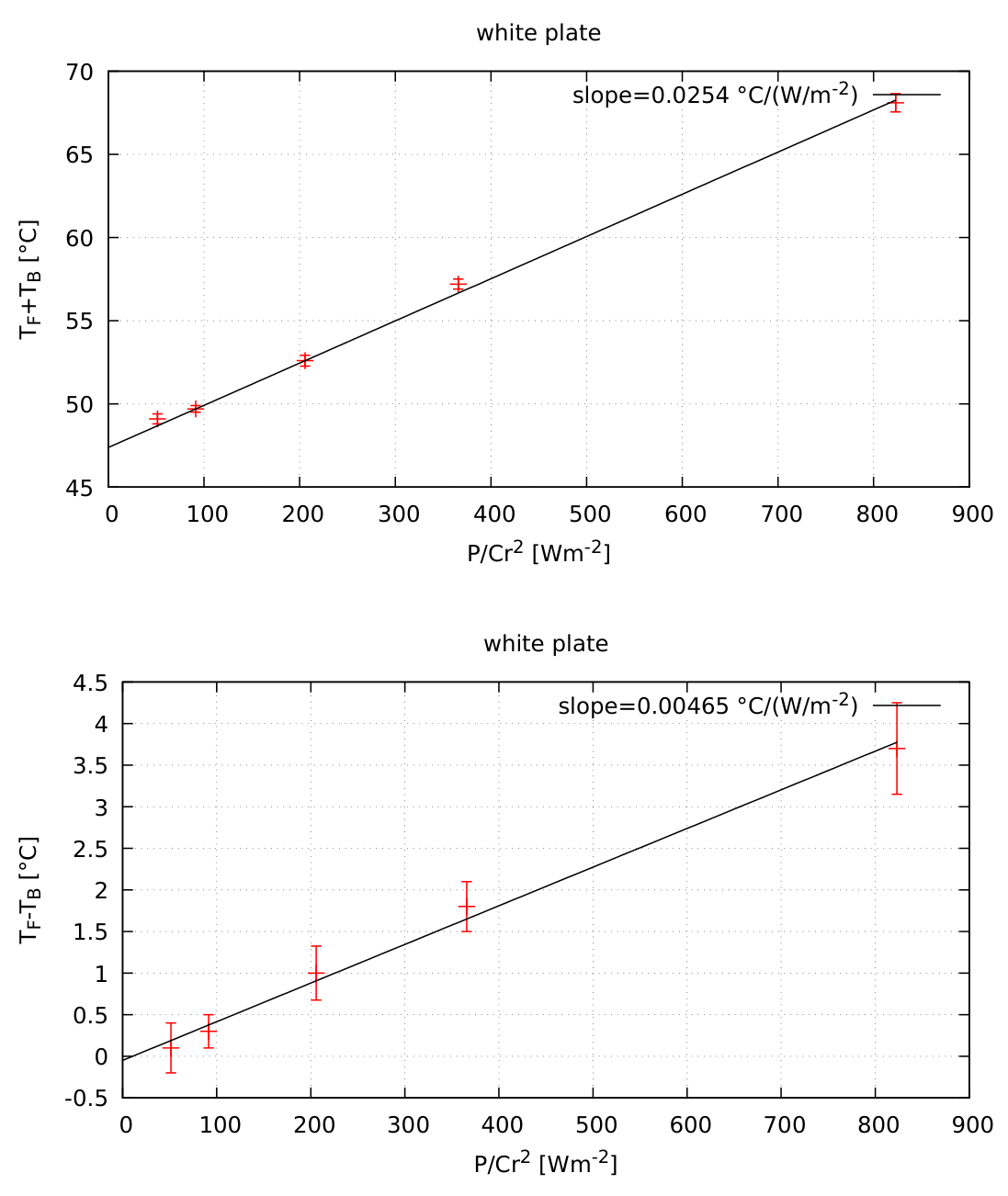
Task 3 (b) Estimate the albedo (the fraction of the irradiance that is reflected instead of absorbed) of the white plastic and perform error analysis.
Useful relations: An area of a segment of a sphere with radius between polar angles and with is .
Picture of equipment
Illuminance table
| [K] | Red [lx] | Green [lx] | Blue [lx] |
|---|---|---|---|
| 1570 | 2 | 0 | 0 |
| 1600 | 4 | 0 | 0 |
| 1610 | 5 | 1 | 0 |
| 1620 | 6 | 2 | 0 |
| 1630 | 8 | 3 | 0 |
| 1640 | 10 | 4 | 0 |
| 1660 | 12 | 5 | 0 |
| 1670 | 14 | 6 | 0 |
| 1700 | 18 | 9 | 1 |
| 1730 | 24 | 14 | 3 |
| 1780 | 37 | 23 | 7 |
| 1820 | 51 | 34 | 11 |
| 1880 | 80 | 57 | 21 |
| 1940 | 120 | 91 | 36 |
| 2000 | 165 | 130 | 53 |
| 2060 | 230 | 194 | 80 |
| 2120 | 310 | 274 | 118 |
| 2160 | 379 | 348 | 155 |
| 2220 | 484 | 460 | 210 |
| 2260 | 586 | 570 | 264 |
| 2310 | 753 | 748 | 348 |
| 2350 | 888 | 929 | 440 |
| 2390 | 1032 | 1107 | 527 |
| 2460 | 1292 | 1452 | 697 |
| 2500 | 1577 | 1826 | 879 |
| 2540 | 1811 | 2198 | 1078 |
Table 1: Illuminances by an incandescent light source of a known temperature, measured through three colour filters at a fixed position of the light source and the light meter. The accuracy of the measurements is lx.
Power supply instructions
The benchtop power supply outputs the maximum amount of electricity allowed by the set current limit and voltage limit. If the current limit is reached first, it operates as a constant current source, and if the voltage limit is reached first, it operates as a constant voltage source, indicated by CC and CV indicator lights.
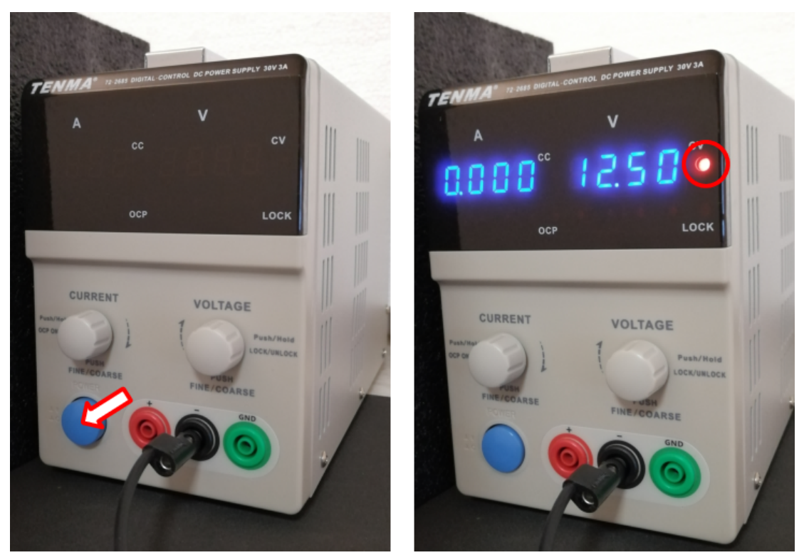
Do not plug in the light source before setting up the power supply! Notice the red wire in the image not connected, so the circuit is interrupted.
You will see two displays: current display on the left and voltage display on the right. They show the actual current and voltage at the moment, so the current will be zero, and the voltage will equal the chosen voltage limit. The CV indicator next to the voltage display will glow, indicating that the voltage limit is reached.
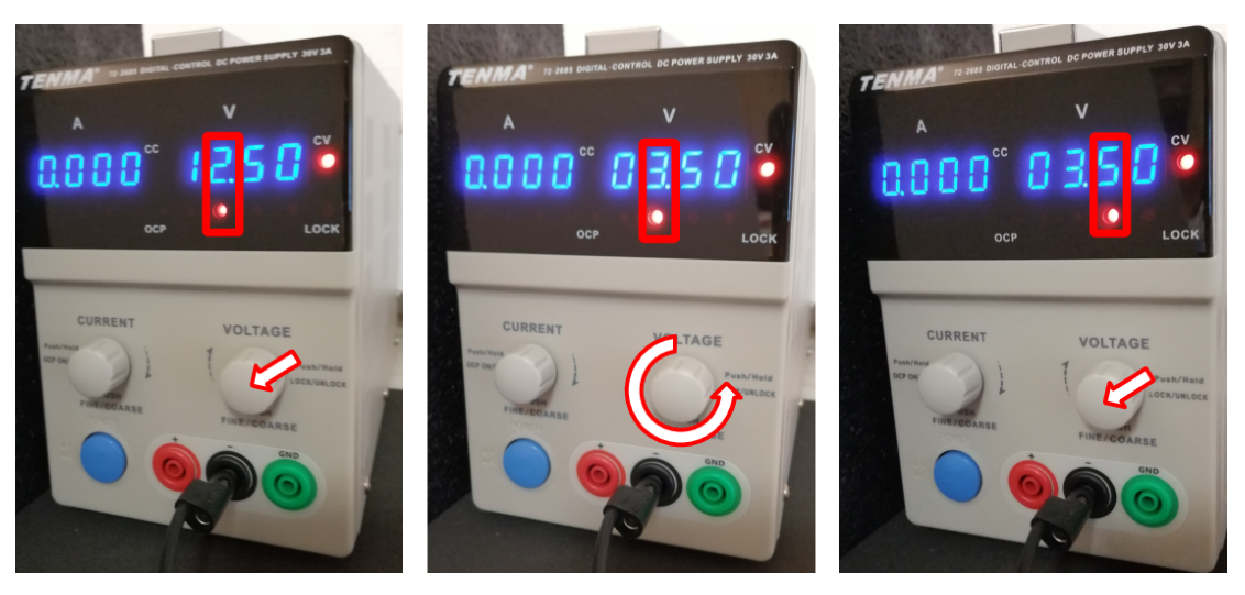
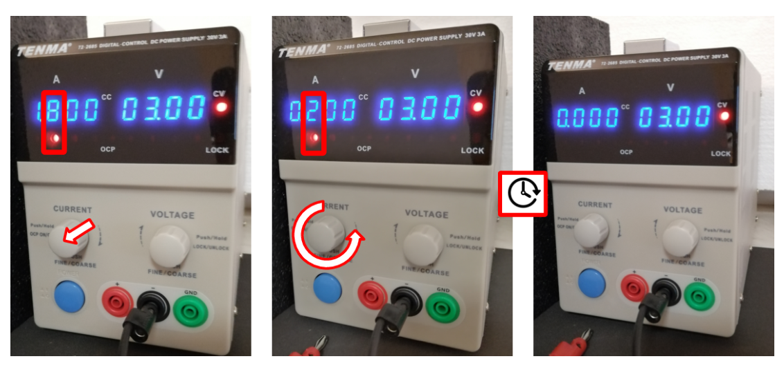
Press the voltage knob to set the voltage limit. The display will now show the voltage limit instead of the actual voltage, and the light below one of the voltage digits will glow. Turning the knob sets the chosen digit, and pressing it will cycle through all the digits. Use this to set the voltage to the maximum allowed voltage of the light source, e.g. for the LED.
After 4 seconds, the display goes back to showing the actual voltage and the light below the voltage digits turns off.
Repeat the procedure with the current knob (left), to set the current limit.
The example shows the limit . After 4 seconds, the display reverts to showing the actual current (still zero), and the digit selector light will turn off.
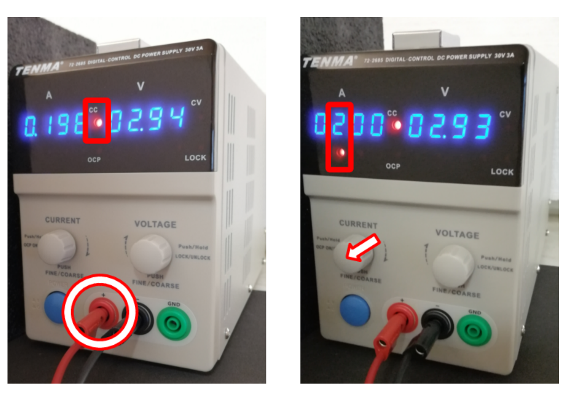
Now that both limits are set correctly, plug in the light source. Now the current limit is reached, indicated by the CC (constant current) light. Actual voltage is now lower than the setting. The light source in this example is not the same as in your experiment, so your values will be different. Try increasing the current limit with the left knob.
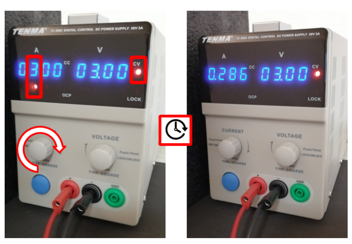
When the current is increased too much, the voltage limit is reached (CV indicator), which protects the light source. Use the current setting to control the light sources.
Отговори
Task 3 (a) Example values in the official solution: h = 10 W m⁻² K⁻¹, λ = 0.072 W m⁻¹ K⁻¹.
The grading scheme accepts h within [10, 14] (full marks) and λ within [0.06, 0.08] (full marks), in SI base units.
Task 3 (b) Example in the official solution: (1 − a) = 0.0254/0.0988 = 0.26 (first graph) and (1 − a) = 0.00465/0.0173 = 0.27 (second graph).
The grading scheme gives full value marks for a ∈ [0.65, 0.75].
Решение
E1: Colour and temperature
Theory
The infrared thermometer cannot be used to measure the filament temperature for several reasons – the range of the IR thermometer (stated on the instrument) only goes up to . The filament is also too small to be the only thing measured. IR opacity of the glass bulb is also not guaranteed. Therefore, the only way to measure the temperature is indirectly through the colour index, for which the relation to temperature is provided.
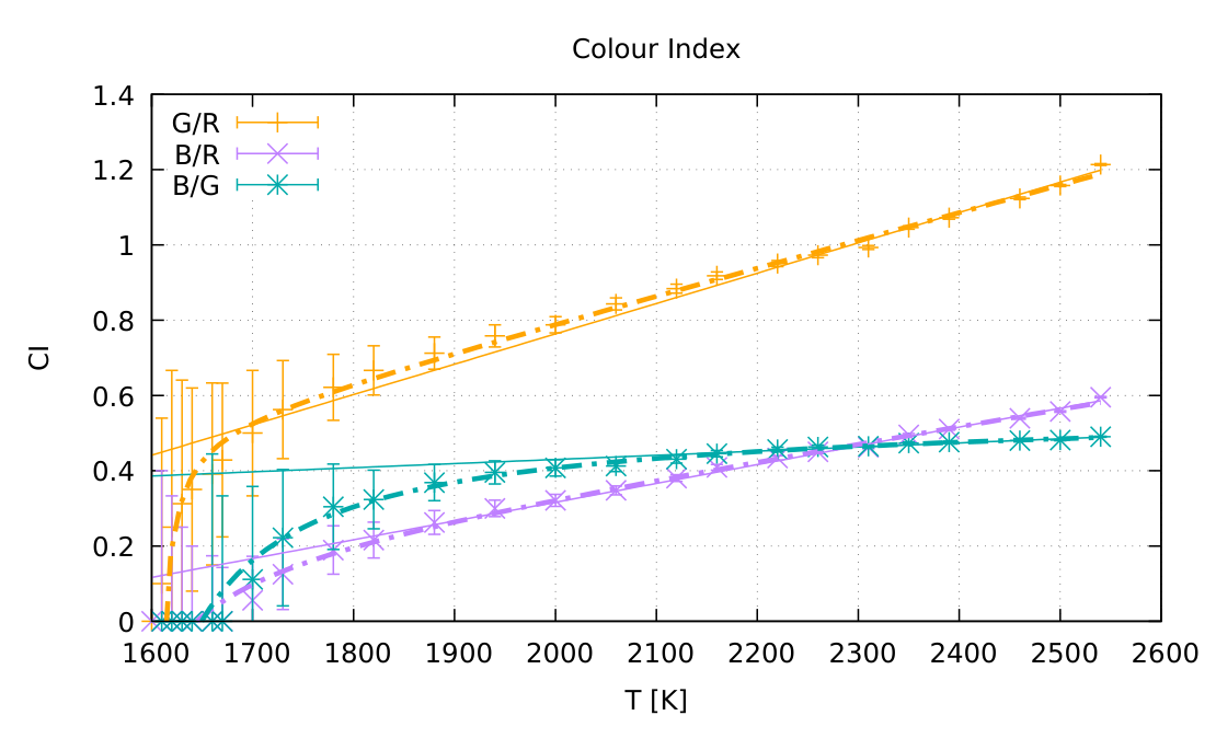
Wien’s displacement law suggests that at lower temperatures, the light will contain more red component than green and blue, while at higher temperatures, the green and then the blue will increase faster than red, leading to increasing ratios , and . We must, however, consider, which pair of filters will be the most suitable choice.
The values measured through different filters depend on the spectral response of each filter, including its overall opacity. It also depends on the sensitivity of the light meter to each wavelength. Instead of theoretical predictions, we are given reference measurements at known temperatures. If we plot the ratios for all three pairs, we observe that is the least suitable, as it changes much less with temperature, compared to the other two. and are comparable, but the blue filter has lower transmittance, which will lead to lower accuracy (higher relative error).
Any pair of filters is a valid choice to proceed with the measurements, but will affect the end accuracy. Averaging the results is also an option, but including combination may still reduce the accuracy of the end result.
To use the plot for converting the colour index to temperature, we need a trend line. A linear trend is enough to cover most of the range, except at lower temperatures, where the relationship tapers off. We can extend the range by combining two trends across the range, or to draw a smooth curve by hand. Zig-zag interpolation is less suitable due to scatter in the reference measurements.
Using the absolute values from the table instead of ratios is not correct, as the intrinsic luminous flux of the light source and the measurement distance are not given.
Experiment
For the measurement of the power dependence of the temperature, we will read out the voltage and current from the power supply. To sample the expected curve of the relationship, we must sample it sufficiently well, especially at lower powers where the temperature changes more quickly. We suggest sampling at least 8 powers/temperatures to cover the relationship more precisely and distinguish outliers from reliable measurements. For each power setting, we must measure the illuminance through the chosen filters by covering the sensor of the light meter with a filter. Covering the light meter filters all the light, including the light reflected from the walls and the floor, leading to a better measurement. Placing the filter next to the light source also introduces the risk of burning the filter. Planning ahead, we can simultaneously measure the illuminances without a filter, needed in Task 2.
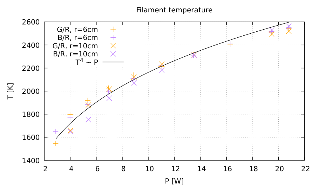
Each colour index is then converted to a temperature by reading out from the calibration graph. We can also estimate the relationship by employing the Stefan-Boltzman law if we neglect other losses and the contribution of the ambient temperature:
According to measurements with multiple light bulbs in different environments, the fit is
which is used as a baseline for determining the RMS of students’ measurements.
The background illuminance must be measured through all filters – it is most likely zero, but a good experimentalist must check, and if significant, it must be subtracted from measurements. This is also a way for us to detect if they left their desk lamp on – if the background differs significantly from the rest of the contestants.
The distance between the light source and the light meter should be short enough to enable accurate measurements at lower powers. Distance can also be different for different power ranges, but care must be taken, as the effect of the finite size of the filament may play a role, as well as the changing reflections from surroundings and from the top of the light stand.
Marking scheme
General guidelines for marking in all tasks
- Granularity for marks is 0.1 p.
- measurements/results given with inappropriate number of significant figures may get deducted 0.1 p. (rule of no propagating error applies)
- A simple numerical error resulting from a typo is punished by 0.1 p unless the grading scheme explicitly says otherwise.
- Errors in theoretical derivations which cause dimensionally wrong results are punished by at least 50% of the marks for the derivation unless the grading scheme explicitly says otherwise.
- Propagating errors are not punished repeatedly unless they either lead to considerable simplifications or wrong results whose validity can easily be checked later.
- Negative points cannot decrease the score under the same section (A1,A2,...) below zero.
| Calibration | Points | |
|---|---|---|
| A1 | Plotting | 1.0 |
| Compute color indices for sufficient number of data points over range | ||
| Plot of color indices | ||
| Proper axis labels & ticks | ||
| Sufficient size of graph for precise readout ( page) | ||
| Each point computed/drawn incorrectly | ||
| A2 | Trend line | 0.5 |
| Smooth trend curve or a composite of linear trends | ||
| Single linear trend line (generates outliers at some temperatures) | or | |
| Zig zag connected points (=used interpolation for readout), or pointwise connected curve | or | |
| Total on Calibration | 1.5 |
This section is only for the calibration data (tables, graphs) based on the given table. Plots made based on IR measurements, get zero points.
Full points are given for a single colour index graph, or for multiple colour indices which may be on the same plot or on the separate plots.
Absolute values plotted: At most points for A1 (if axes and ticks are done correctly, see the table above), if they plotted the absolute values through one filter or differences of values of several filters, instead of colour indices. The illuminance depends on the distance and the brightness of the light source, so absolute values cannot be used to determine the temperature. Points for A2 may nevertheless be given.
| Measurements | Points | |
|---|---|---|
| B1 | Data collection † | 1.2 |
| Measured , , through 2 or 3 filters at points (for 1 filter only and rounded, for measurement of and or RG(B) only, which typically happens with measurements with IR thermometer, max. 0.3) | ||
| Compute | ||
| Compute color indices or convert directly to temperature (from graph or trend in A2) | ||
| No points below | ||
| No points above | ||
| Measured RGB background | ||
| Determined background constancy (e.g. measured at the beginning and the end) | ||
| B2 | Temperature plot ‡ | 0.9 |
| Determine temperatures | ||
| Plot of data | ||
| Add best fit curve | ||
| Proper axis labels & ticks | ||
| Proper size of graph | ||
| Each point determined/drawn incorrectly | ||
| Used G/B index | ||
| B3 | Result quality ‡ | 0.4 |
| Nonlinearity of the relationship is visible | ||
| Nonmonotonous relationship | ||
| RMS from best fit within | ||
| RMS from best fit within | or | |
| RMS from best fit within | or | |
| Total on Measurements | 2.5 |
† Presentation of data: If and are directly multiplied and only values are presented, no marks are deducted.
Background: Points for background are only granted if the background is subtracted from the measurements, or can be reasonably neglected.
‡ IR measurement: If temperatures are “determined” from IR measurements or any other method unfit to determine the temperature, no marks are given for B2. The same holds for B3, because presence of nonlinearity is not an indicator of quality for meaningless data.
To determine the RMS at B3, we compare it to Eq. 2 and take the root of the mean squared deviation. Reasonably exclude any outlying measurements at very low powers where we expect large deviations. The RMS calculations can be handled by the auxiliary Excel file.
E2: Efficacy
Theory
Light sources do not radiate in all directions equally. The angular distribution of luminous flux (luminous intensity) must be integrated over the solid angle. A light meter at distance to the light source, oriented so that the light falls on it perpendicularly, measures the illuminance of a certain part of the imagined integration sphere surrounding the light source:
The LED only shines the light into a hemisphere, and has cylindrical symmetry around the direction straight ahead, so we can simplify the expression,
and for the incandescent bulb, the symmetry axis is perpendicular to the direction straight ahead, and shines into full solid angle:
The integrals will have to be evaluated numerically – it can be done by using the trapezoidal or the Simpson method, or by using the formula for a spherical segment area given in the hint:
and equivalent (but with sin cos) for the incandescent bulb. Here, choosing evaluation points in the middles of intervals is better than choosing one of the edge points. However, the exception are the “edge” measurements, where the measurement point is actually in the middle of the interval – the point straight ahead for the LED is in the middle of the spherical cap. The same goes for the “poles” of the incandescent light bulb.
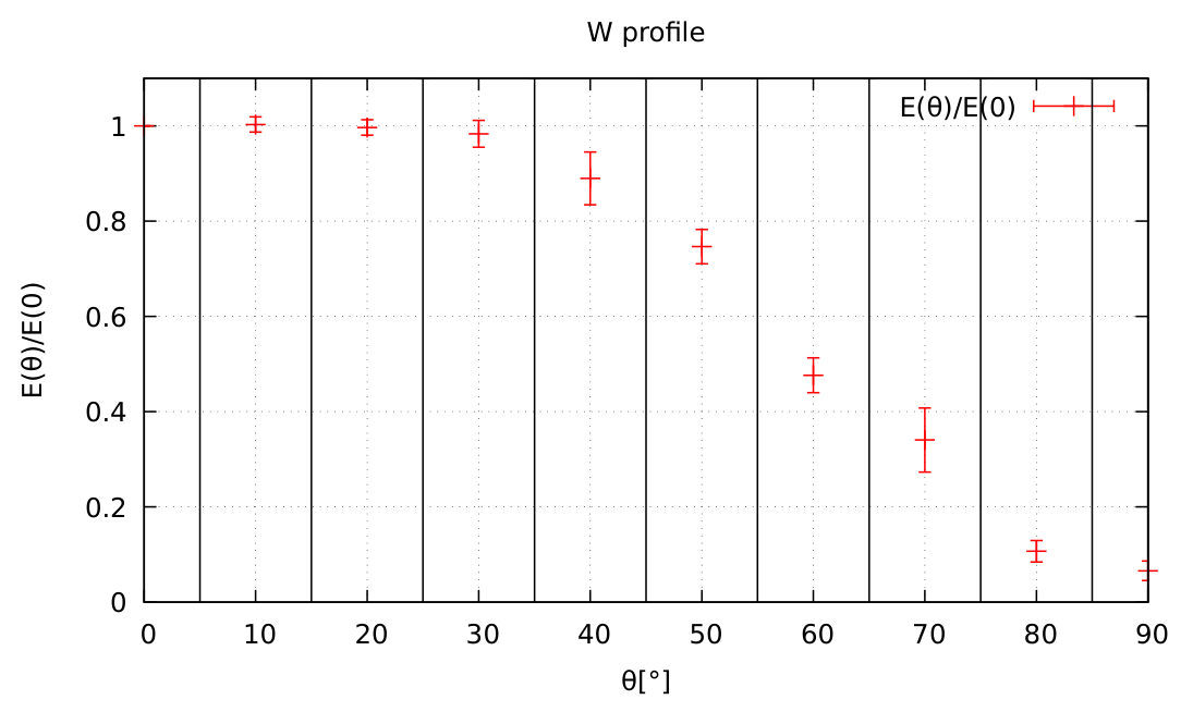
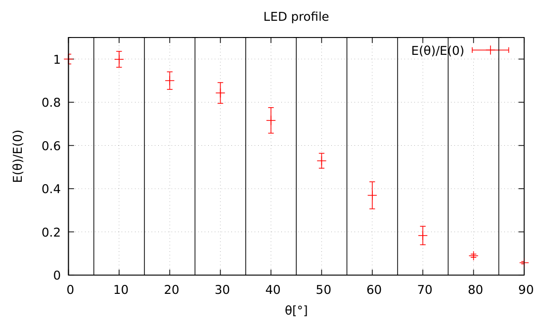
The ratio between the head-on measured illuminance and the luminous flux, can be expressed as
or, more intuitively, as a correction factor to the isotropic source:
Analytical estimates
One possible pathway is to estimate these factors without measurements, using reasonable assumptions about the light distribution. The LED can be assumed a planar emitter, with a cosine distribution of luminous flux:
which turns out to match the experiment well.
For the incandescent bulb, a similar assumption can be made based on a thin filament model. The different orientation of the symmetry axis leads to a different result:
These approximations can be used to a good effect but are not required in the experimental task.
Experiment
To measure the angular dependence, a suitable distance to the light source must be chosen. Too far, and the signal becomes weak and any background could become noticeable. It is advisable to measure the angular dependence at the highest power in order to improve the signal to background ratio. Measurement can also be performed through one of the filters.
For the incandescent bulb, the finite size of the filament becomes an issue if we measure too close to the bulb. This becomes noticeable at distances lower than . This was not an issue for the colour index measurement, but it matters for the absolute flux estimation.
To describe the inflection point in the light distribution well, we will need at least measurements in the interval. We can either rotate the light source on the spot, or position the light meter at different angles in relation to the stationary light source.
For the light distribution left-right symmetry can be assumed, or, alternatively, the entire range can be measured, allowing to take into account asymmetries and an angular offset in the light distribution. The straight ahead measurement is centered in a symmetric band, which needs care so it is not double-counted in case only half of the range is integrated and then doubled.
With the conversion factors known, the luminous efficacy can be determined by measuring the frontal illuminance at powers that cover the entire range from the lowest detectable illuminance to the maximum allowed power. For the incandescent bulb, this measurement can be done simultaneously with Task 1 for better time efficiency.
| W | ||
| LED |
Table 1: Example values of the conversion factor between the frontally measured illuminance and the luminous flux for both light sources. The values will vary within some wider distribution because of varying light sources and other errors, which is indicated by the brackets in the grading sheet.
It is not required to measure at the same distance as the angular dependence. Multiple distances may also be used.
We have to avoid placing any additional objects near the light source to avoid introducing more reflected or blocked light – such as placing the light source directly on the white paper, or having other obstructions such as the black paper screen or any filters too close to the light bulb.
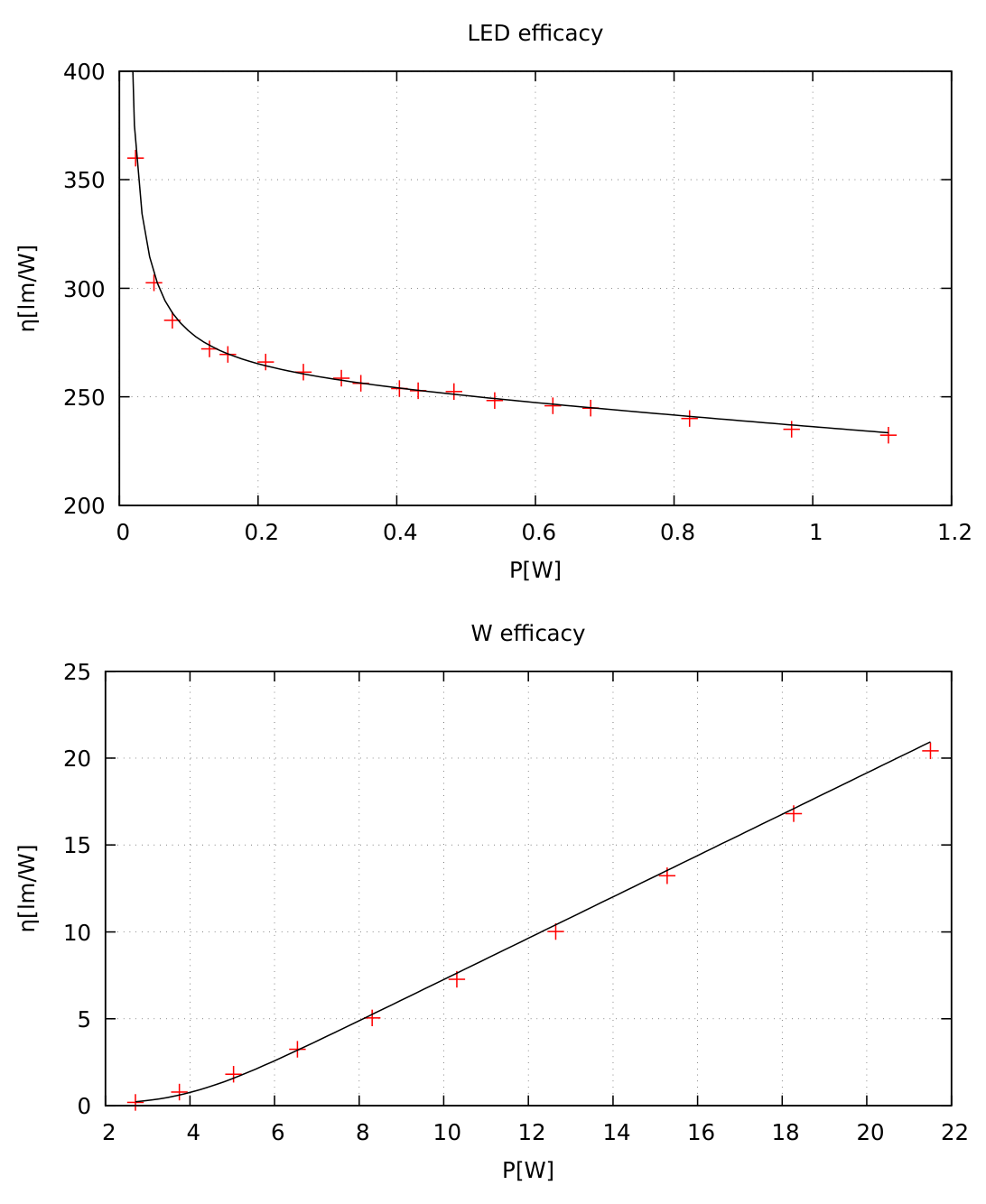
To plot the efficacy, we divide the obtained from eq. (3) for each of the light sources, with read out from the power supply.
The result shows that the efficacy of the incandescent light starts out at zero at low powers and increasing with power, as its temperature increases. The LED has the highest efficacy at lowest powers, then it drops off at higher powers, mostly due to increased temperature of the light emitting junction.
At the lowest settable currents, the readout on the power source is no longer reliable – for example, LED may glow slightly even at . The pole at the origin can be attributed to this source of error.
Marking scheme
The basic equations could be stated in a separate section of the solution, or spread over different parts of the solution.
| Theoretical background | Points | |
|---|---|---|
| A1 | Eq. (3) or equivalent | 0.5 |
| Dependence on | ||
| Dependence on angle (noticing anisotropy) | ||
| A2 | Take into account cylindrical symmetry (each) | |
| Choose right symmetry axis for light sources (each) | ||
| Correct factors of and (LED and bulb, respectively) | ||
| Assume area of the sensor comes into calculations | ||
| Total on Theory | 1.0 |
means one for each light source (bulb, LED).
| Angular measurement | Points | |
|---|---|---|
| B1 | Incandescent measurement | 0.9 |
| Measured at or more angles between and | ||
| Specified auxiliary data (power, distance) | ||
| Measured full angular range (e.g. by rotating light) | ||
| Maximum illuminance below | ||
| Measured closer than | ||
| B2 | Integration procedure | 0.7 |
| Used the hint | 0.7 | |
| Values at the edges of intervals | ||
| Double counting of the equator | ||
| Used trapezoidal or similar rule | or | |
| Incorrect treatment of edge values | ||
| Double counting of the equator | ||
| Analytically derived eq. (10) or similar | or | |
| Averaged values without weights | or | |
| B3 | result accuracy for Tungsten | 0.3 |
| Calculated or equivalent | ||
| Value of | ||
| Value of | or | |
| B4 | LED angular measurement | 0.9 |
| Measured at or more angles between and | ||
| Specified auxiliary data (power, distance) | ||
| Measured full angular range (e.g. by rotating light) | ||
| Maximum illuminance below | ||
| B5 | Integration same as B2 | 0.7 |
| B6 | result accuracy for LED | 0.3 |
| Calculated or equivalent | ||
| Value of | ||
| Value of | or | |
| B7 | Background measured | |
| Background constancy check (multiple measurements) | ||
| Total on Angular | 4.0 |
Plotting the angular dependence is not required for the procedure, but it counts as points if the integration procedure was otherwise not performed.
If a matching analytical value for both conversions are obtained, but angular dependence is not measured, the contestant can get all marks except for the measurement ( out of for each light source).
If a comparison of analytical and experimental estimate are done, or if an analytical model is fitted to the experimental data, the procedure is correct, and up to additional points per light source may be given to compensate points lost for steps that merit points that may not be necessary for the method used.
| Efficacy measurement | Points | |
|---|---|---|
| C1 | Incandescent measurement | 0.7 |
| Measured , , for incandescent light at points | ||
| No measurements above | ||
| C2 | Plotting bulb efficacy | 0.8 |
| Convert and plot points (if converted into flux, not efficacy max ) | ||
| Missing axis labels | ||
| Deviation from a monotonous shape | ||
| † | Values within RMS | |
| Values within RMS | or | |
| C3 | LED measurement | 0.7 |
| Measured , , for LED at points | ||
| Fewer than 2 measurements above | ||
| Fewer than measurements below | ||
| C4 | Plotting LED efficacy | 0.8 |
| Convert and plot points (if converted into flux, not efficacy max ) | ||
| Missing axis labels | ||
| Deviation from a monotonous shape | ||
| ‡ | Values within RMS | |
| Values within RMS | or | |
| Total on Efficacy | 3.0 |
† Vary the factor within the range to check for a better match. This helps remove propagation error from a badly determined and additionally, any small variations in power output between light bulbs.
‡ Vary the factor within the range to check if there is a better match. The LEDs may vary in light distribution and absolute intensity, so the trend cannot be matched 1:1. Exclude also the lowest power outliers from the assessment, as the singularity can give a high RMS without being significant to the LED itself. It depends on the voltage bias of the power source and resistivity of junctions.
RMS comparison: To make the comparison of the graphed solutions to the reference less subjective, we do a root mean square comparison: average square deviation from an empirical model curve based on a larger number of measurements in a controlled environment (Fig. 5). For the light bulb efficacy, we use
which is just a linear function smoothly flattened at the bottom.
For the LED, we use
where possible intensity variations can be compensated by allowing variation in C2/C4. Variations in the part (due to different offsets in power supply readout) can be compensated by excluding the low-power measurements from the RMS calculations in a reasonable way.
All these are in base units without prefixes (omitted for clarity).
If angular dependence is ignored use this table as a shortcut for grading
| A1 | dependence on only | |
| A2 | Correct factor of or only | |
| B1-B6 | not applicable | |
| B7 | Background measured | |
| Background constancy check (multiple measurements) | ||
| C1 | No change | |
| C2 | Rescale with correct to check RMS | |
| C3 | No change | |
| C4 | Rescale with correct to check RMS |
E3: Radiative heating
Theory
The plate receives a radiant flux density , determined by the power of the light source, and the distance between the target and the light source. The light source does not shine equal amounts of light in all directions, therefore we must use the correction factor , derived in Task 2, to convert from the total radiant flux to forward radiant flux density.
Not necessary, but also correct, is to (numerically) integrate/average across the entire plate, to take into account spatial variation of , and (angle of incidence).
The incident flux density is dissipated to the environment directly, as well as by heat conduction through the plate. Mark by the front temperature and the back temperature. Conservation of energy gives us the system of equations
This system of equations leads to the following relations:
Any linear combination of equations (14,15) also allows determination of both and . A particular linear combination that may be used is the isolation of individual temperatures:
In our system, , but still in the same order of magnitude. Treating the slope of as or the slope of as is a reasonable approximation, but still not theoretically correct.
Error analysis
Errors should be propagated from the slope. For example, if they obtain slopes and , they should propagate the errors. We should allow both straight addition of error contributions of different terms, or adding squared errors (independent errors), e.g.
and analogously for other slope definitions.
Albedo
For the white plate, only a part of the incident flux is absorbed, so we replace by if is the albedo:
As a consequence, any slope measured for both plates will be in the ratio to each other. This can be expressed as a fraction of trend slopes, ratio of temperature differences, or similar.
Experiment
The radiant flux density can be varied in two main ways, or a combination of both: by changing the distance, or by changing the current through the light bulb. Both methods are acceptable, but varying the current also changes the spectrum and the efficiency of the light bulb, so it may produce biased and nonlinear results. The students should know that varying a single parameter is the correct procedure.
The required measurements in this task are the front and back temperature at different powers, for black and white plate. It is essential to wait for equilibration, which includes waiting the back temperature to stabilize. It is advisable to measure starting with the lowest flux density, because it will require the least equilibration time from the initial room temperature of the plate.
The target should not be too close to the light source, not only because of the risk of burning, but also because close to the light bulb, the light is very nonuniformly distributed across the plate. Increased convection rate due to high temperature also starts deviating from the linear regime. Placing the target too far from the light source leads to a negligible heating and thus a very large relative error in temperature differences, especially for the white plate.
In this task, the measurements are subject to many sources of errors: measuring from different distances and at different angles may include different proportions of background or reflected IR radiation from the light source (if the targeted area is still illuminated), if the measurement takes too long, the plate may start cooling down (this is noticeable in a few seconds), air currents may increase convective heat dissipation, and the ambient temperature may also change during the measurement (especially if the light source is placed too close to the wall, or if the power source’s fan exhaust is too close to the measurement setup). The errors are most noticeable at low radiant flux and for the white plate, where increases in temperature are the smallest.
For these reasons, it is advisable to take more than one measurement per data point and average the results, and to cover a sufficiently wide range to reduce the slope error. At least points are needed to draw a trend, but is better. With more points, it is easier to spot outliers and utilise the measurements which are least subjected to errors. Back and front temperatures are best measured in pairs one after the other to reduce the error in the temperature difference signal due to changing conditions.
Note: the ambient temperature is an effective temperature that combines air temperature and radiative exchange with the surrounding walls, ceiling and other objects. We do not need its value, we only need the slopes of the linear trends. Inexact can lead to inaccuracies if used together with an assumption the linear relations go through the origin. cannot be reliably determined by measuring surrounding temperatures, but it can be estimated by measuring the equilibrium temperature of the plate in the absence of the light source.
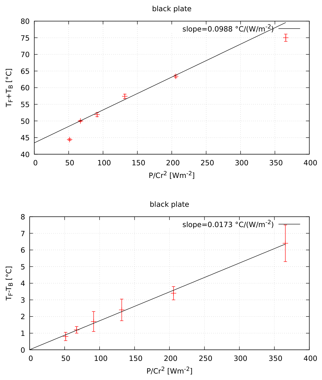
The measurements of the front and back temperature at different radiant fluxes, must be processed and plotted to extract the necessary slopes. For the black plate, two plots will be needed, based on equations (14,15), equations (16,17), or any linearly independent pair. Linear regression gives us the slopes and (or their reciprocals). is best determined by the intercept of the trend line for (Eq. 16) or any equivalent plot, and should match determined by other methods. If measured correctly, the intercept of the trend line for (Eq. 17) should be zero within the error margin.
It is possible to calculate the necessary slopes from a measurement at a single input power (for each plate color), if is measured well. This can be done without a graph. However, using multiple measurements decreases the impact of statistical errors and enables us to better estimate the error, so a single measurement will carry a significant error.
Albedo, as defined in the task text through irradiance units, cannot be measured using a light meter, which measures in photometric units. Additionally, light reflected from a white plate introduces additional geometric considerations and angular distribution of reflected light, that cannot easily be taken into account.
The albedo can be estimated as a fraction of the corresponding line slopes between the black and the white plate, taking any of the relations (14,15,16,17). This means that for the white plate, measuring only one side of the plate is enough to determine the albedo, assuming and remain the same. The difference slope or the back temperature slope are the least suitable, as they introduce a large relative error to the measurement due to a minimal increase in temperature.
Marking scheme
The basic equations could be stated in a separate section of the solution, or spread over different parts of the solution.
| Theoretical background | Points | |
|---|---|---|
| A1 | Power to irradiance | 0.4 |
| Correct eq. (13) or equivalent | ||
| Realizing the same geometry from Task 2 applies ( or equivalent) | ||
| A2 | Heat exchange balance | 0.6 |
| Correct each of eqs. (14,15) or equivalent. | ||
| Each partially correct eq., e.g. assumed in (14) or missing or in (17) | or | |
| A3 | Albedo balance | 0.2 |
| Correct eq. (22) or equivalent | ||
| Total on Theory | 1.2 |
The assumption that the left hand side of equation distributes the full power of the light source to the area of the plate, indicates a lack of understanding and merits points for theory part.
If conduction is not considered at all a maximum of 0.1 points is given to A2.
| Measurements | Points | |
|---|---|---|
| B1 | measurements of (black) | |
| B2 | measurements of (black) | |
| B3 | measurements of , or both (white) | |
| B4 | Measured the unchanging values (distance if varied, if distance varied) | |
| Estimated measurement errors (at least separate for each plate color) – the instrument precision is not a valid error estimate | ||
| Estimated measurement errors (common for all) | or | |
| Measured by varying the current (not distance) | ||
| Total on Dissipation | 1.9 |
Determination of and will require extraction of two trend lines from two plots. Plotting on the same graph counts as two, but the vertical axes must be labelled correctly. The trend lines will have a intercept that will be in case of temperature difference, and related to ambient temperature otherwise. Using or instead of as an axis is valid as long as the conversion is done correctly at the slope readout.
| Dissipation parameters | Points | |
|---|---|---|
| C1 | First of the two plots | 0.8 |
| correctly converted and drawn points | ||
| Correct trend line | ||
| Correct slope readout | ||
| Slope error estimate | ||
| Intercept disagrees with expectations | ||
| Missing axis labels, ticks or unsuitable size | ||
| C2 | Second of the two plots | 0.8 |
| Same breakdown as C1 | ||
| C3 | Calculation of | 0.8 |
| Correct algebraic relation to slopes | ||
| Numerical value within | ||
| Numerical value within | or | |
| Numerical value within | or | |
| Correct error analysis | ||
| Error estimate (if error analysis is reasonable) | ||
| C4 | Calculation of | 0.8 |
| Correct algebraic relation to slopes | ||
| Numerical value within | ||
| Numerical value within | or | |
| Numerical value within | or | |
| Correct error analysis | ||
| Error estimate (if error analysis is reasonable) | ||
| Total on Dissipation | 3.2 |
The values are in SI base units.
Without plotting: If the entire fitting process is done numerically without plotting, use equivalent concepts to the grading above – tables instead of plots, slope calculations instead of trend lines, etc. As the plot is not required, a correct procedure can yield full points.
The error analysis in this case may consist of doing the entire procedure (e.g. using a single measurement with knowledge, or two points without background), with multiple measurement runs and doing statistics. Another option is propagating relative errors from the single measurement errors. The main criterion is, that the error source is statistical, not instrumental.
The point count includes the origin for the plot of the temperature difference (eq. 17).
The slope error is the main source of error – distances and powers can be considered accurate. Error estimate on the slope can be done based on point scatter (but not with fewer than 5 points), with or without taking into account errorbars (if the students estimated them).
Error propagation: if a wrong value of is used, recalculate with a suitable value and grade accordingly.
| Albedo | Points | |
|---|---|---|
| D1 | One or more plots | 1.0 |
| correctly converted and drawn points | ||
| Estimated individual measurement error | ||
| Correct trend line(s) | ||
| Correct slope readout | ||
| Slope error estimate | ||
| Intercept disagrees with expectations | ||
| Missing axis labels | ||
| D2 | Data processing | 0.7 |
| Correct algebraic expression for | ||
| Numerical value | ||
| Numerical value | or | |
| Correct error analysis | ||
| Error estimate (if error analysis is reasonable) | ||
| Total on Albedo | 1.7 |
The possibility of measuring both temperatures allows combinations where both sets of data can be used for albedo estimation – by averaging two slope ratios, or similar. This is also a valid approach.
In cases where only pointwise numerical evaluation using several data points is employed a maximum of 0.5 points for D1 (0.3 conversion of data, 0.2 for error estimates) and a maximum of 0.7 for D2 will be awarded. For evaluation with one data point only a maximum of 0.2 points for D1 (0.1 for conversion of data, 0.1 for error estimate) and 0.5 for D2 (0.2 algebraic expression, 0.2 value, 0.1 error analysis) will be awarded.
Оригинал в Архива: Experiment.pdf · официални решения: Experiment Solutions.pdf