Съдържание
УсловиеTask E1: Probing the acoustic field (1 т.)Task E2: Acoustic levitator properties (4 т.)Task E3: Density of solid beads (3 т.)Task E4: Evaporation (3 т.)Task E5: Surface tension (2,5 т.)Task E6: Explosion (4 т.)Task E7: Mysterious line (2,5 т.)Task E8: Intentional damage penalty (-0,5 т.)EquipmentРешениеEuPhO 2026, Експеримент — Задача 1. Acoustic levitation
Experimental task Language: English · 20 т.
Условие
An acoustic levitator consists of transducers which convert an electrical signal into intense sound waves. The acoustic pressure of the resulting interference pattern can levitate small objects close to the nodes of the pattern.
Warning: Avoid short-circuiting the connections on the top and bottom of the levitator.
The tasks E1-E7 of this exam are designed to be independent of each other's results. You may skip tasks you are struggling with.
For the following tasks, consider only the nodes on the z-axis. For task E3 and onward, use only the centremost node. The Mode X switch on the electrical box (F), see Fig. 1, should be in position O.
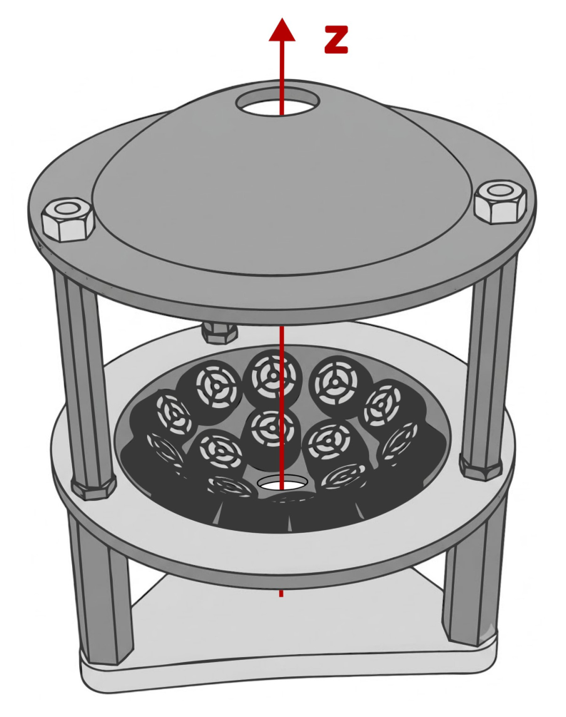
Task E1: Probing the acoustic field (1 т.)
To get familiar with the acoustic field, use the green LEDs (A) and the transducer (B) to construct a tool that emits light according to the local acoustic intensity. A transducer is a capacitor whose charge depends on the mechanical pressure applied to it.
a) Draw a circuit diagram for your tool. [0,5 т.]
b) Use your tool to roughly estimate the distance between two adjacent antinodes on the axis in the centre of the levitator. [0,5 т.]
Task E2: Acoustic levitator properties (4 т.)
In what follows, to levitate a small solid object, the voltage of the connected power supply can be initially put to a high voltage, for example 17 V. The object can be placed in the nodes by using the tweezers. Note that the levitating object can oscillate horizontally due to air-turbulence; wait a little for things to settle. Small oscillations are not detrimental to measurement results.
a) Design, sketch and use a setup to determine as precisely as possible the frequency of the transducers. The speed of sound in air is . [2 т.]
b) Switch Mode X to position I on the electrical box (F) to change to a different mode of operation where the transducers in the upper half of the levitator are supplied with a slightly different frequency than the lower one. Describe the changed behaviour of the levitated objects in this mode and determine the frequency difference and its sign. [2 т.]
Remember to return the Mode X switch to position O for the rest of the exam.
Task E3: Density of solid beads (3 т.)
Levitated objects will be situated slightly below the node due to gravity. The restoring acoustic force acting on the levitated object is proportional to , where is the acoustic pressure amplitude at the antinodes and is the voltage from the power source.
Experimentally determine the density of the unknown beads (O) as precisely as possible. The density of the glass beads (P) is . These spherical beads (O, P) have the same size.
Hint: Depending on your approach, for spherical objects and small displacements from the node, you may use the approximation:
Here, is some unknown function of the radius of the levitated object.
Task E4: Evaporation (3 т.)
For the remaining tasks, you will levitate liquids, which will form small droplets in the nodes. Place droplets in the levitator using the syringes (R) with needles (S). To avoid cross-contamination, use a separate syringe for each liquid. A good starting voltage for most droplet sizes is 8–12 V; at higher voltages the droplets may explode.
Warning: Avoid spilling liquids on the electronics and the transducers. Keep the metal net (L) on the bottom of the levitator; if it gets wet, remove it and let it dry. If the transducers seem to malfunction, raise your HELP sign.
The exact shape of the levitated droplets can be complicated. Moderately deformed droplets may be approximated as an ellipsoid with semi-axes , which has the volume:
In this task, you will study the evaporation of a liquid droplet in the levitator. A simplified description for the evaporation of a droplet with equivalent diameter is given by:
where is the equivalent diameter of the droplet, i.e., the diameter of a sphere with the same volume as the real droplet, and is the evaporation constant. For this task, consider only liquid I and keep the voltage constant.
a) Determine the evaporation constant in units for droplets with an equivalent diameter . [2,5 т.]
b) Would you over- or underestimate the time it takes for a droplet to evaporate entirely, using your result from a)? [0,5 т.]
Task E5: Surface tension (2,5 т.)
The shape of the droplet depends only on its volume and the ratio . Here, is the surface tension of the liquid.
a) Perform a measurement to find out which liquid, I or II, has a lower surface tension. [0,5 т.]
b) Experimentally determine the surface tension of liquid I, given that the surface tension of liquid II is . [2 т.]
Task E6: Explosion (4 т.)
When the acoustic pressure is too high, the levitating droplet will explode. A theoretical formula for the maximum voltage that can be applied to the droplet before it explodes is:
where and are some constants.
Consider only liquid II for this task.
a) Determine the constants and in the units and , respectively. [2 т.]
b) Estimate the maximum diameter of a droplet that can be levitated. [2 т.]
Task E7: Mysterious line (2,5 т.)
When the levitating droplet becomes rather flat, a levitator voltage can be found for which the light from the red LED passing through the droplet forms a sharp horizontal line on the screen behind.
Consider only liquid III for this task.
Draw a sketch of the ray propagation inside the droplet when the line appears. Use the line phenomenon described above to estimate the refractive index of liquid III.
Hint: For the line to be visible, the LED must be well aligned with the droplet, see Fig. 2.
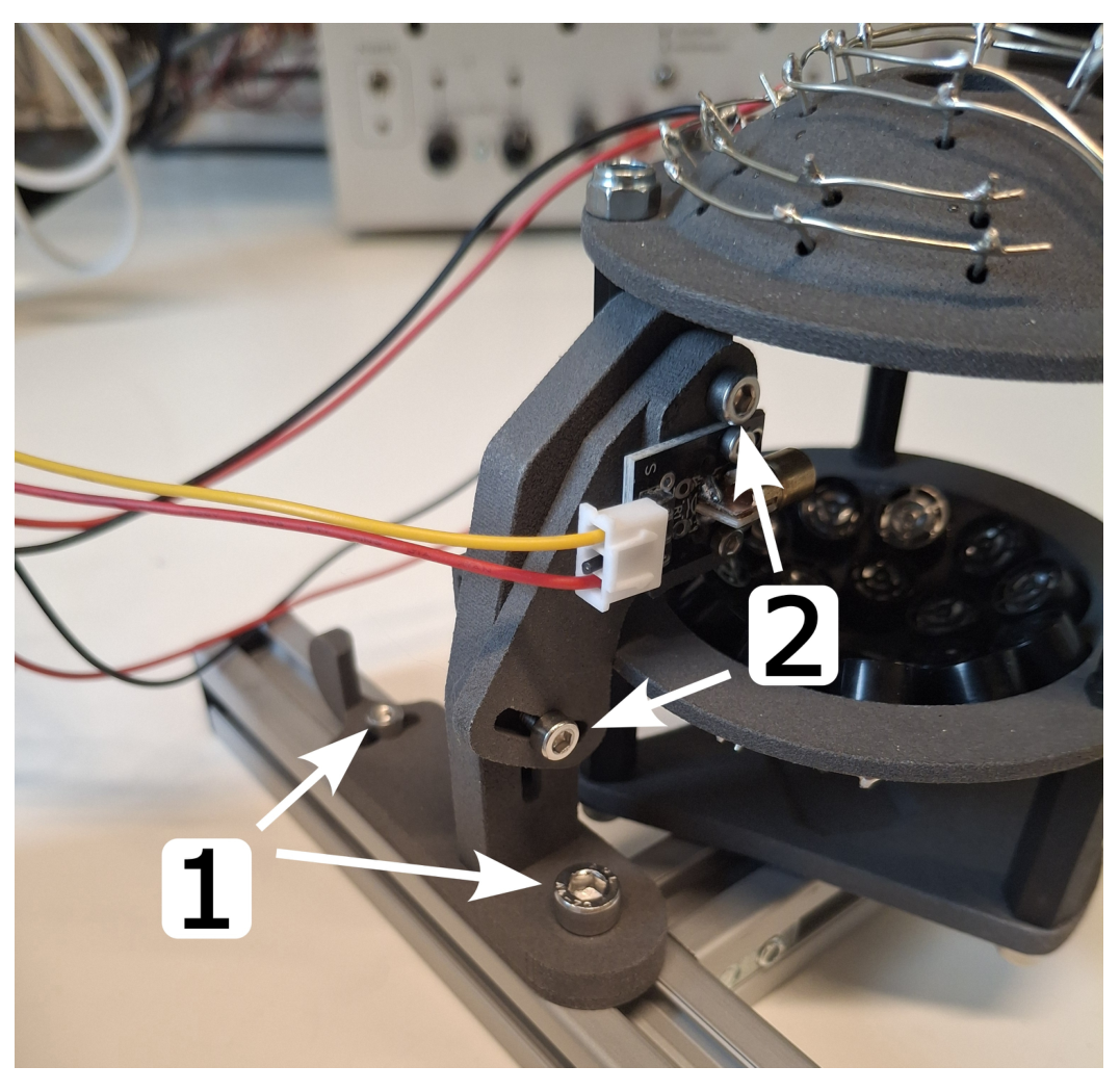
Task E8: Intentional damage penalty (-0,5 т.)
All equipment and packaging is left on the table after the competition in working condition. For breaking components or packaging due to careless handling or failing to follow the warning in red text, a penalty will be applied. (-0.5 pts)
Equipment
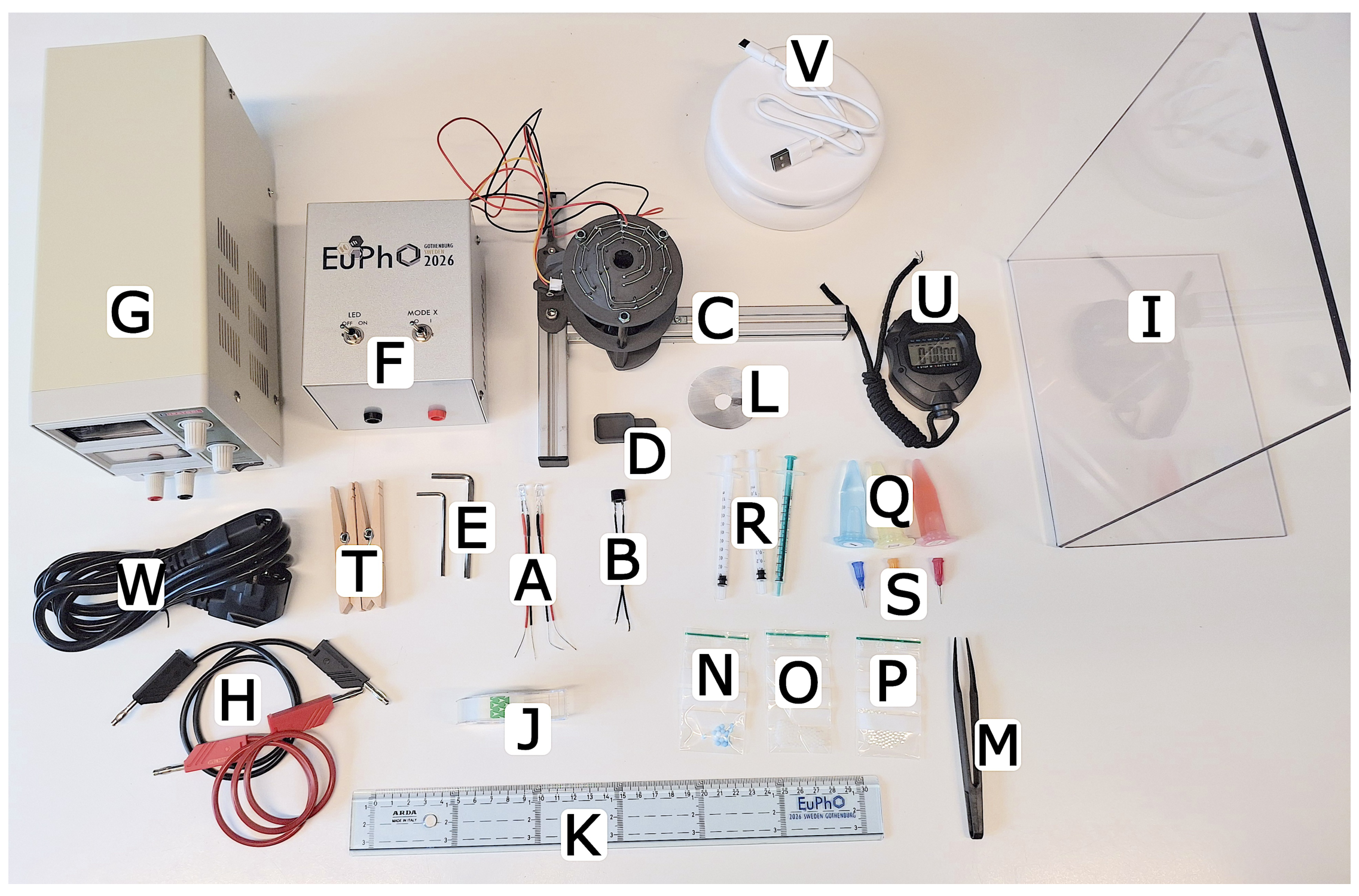
A. Two green Light Emitting Diodes (LEDs). Do not connect the LEDs to the power supply (G).
B. Individual transducer.
C. Metal frame with a levitator module and a red LED, which can be modeled as a point source.
D. Capture unit for collecting falling objects.
E. 2 hex keys for mounting and aligning the setup.
F. Electrical enclosure with switches LED and Mode X.
G. Power supply.
H. Banana cables.
I. Screen.
J. Tape.
K. Transparent ruler.
L. Metal net.
M. Tweezers.
N. 15 blue styrofoam beads.
O. Multiple white spherical beads of unknown material (⌀ 2.0 mm).
P. Multiple transparent spherical glass beads (⌀ 2.0 mm, ).
Q. 3 different unknown liquids labelled I, II and III. They are all safe to touch with your hands, but should not be ingested.
R. 3 syringes.
S. 3 blunt end needles for the syringes (be careful!).
T. 2 clothes pegs.
U. Stop watch.
V. Lamp.
W. Power cord.
X. Piece of paper to dry the metal net (not in image).
If you suspect that a component has failed for some reason during the competition, inform the invigilator to get help.
Решение
General grading instructions:
- Common small penalties
- Missing units in measurements, only penalized once per subtask. -0.1 pts
- Solution in different units than asked: -0.1 pts
- Minor arithmetic error: -0.1 pts
- When graphically evaluating data - using less than half the area on graph paper for plots: -0.1 pts
- When grading numerical results, we do not award points for correct values achieved by guessing (e.g. just stating ), without a effective measurement method presented and raw data recorded.
- When determining the parameters from a linear fit, both a graphical solution as well as using a linear regression on a permitted calculator can be awarded full points for data evaluation. However in the latter case, it is necessary to state that a linear regression on a calculator was used and all raw data used must be presented in a table on paper.
- For all items in a grading scheme, we only award either the full points for this item-ID, zero points, or specified partial points. We avoid awarding non-documented partial points.
- The two grading items E2-A3 and E2-A4 labeled with GLOBAL can be awarded for a criterion fulfilled in the specific subtask or anywhere else in the exam.
Överkurs, i.e. extra information
All solutions are given as a numerical result ± two statistical standard deviations, and all possible systematic errors are ignored. This is not required by the students.
Task E1: Probing the acoustic field
a) Circuit diagram
The transducers in the levitator act as transmitters and are arranged such that a standing acoustic field with pressure nodes and antinodes is created. In the nodes, the pressure variation is minimal due to destructive interference, whereas in the antinodes it oscillates most strongly. An additional transducer can be used as a receiver to probe this field and convert the pressure differences into an alternating voltage. This spatial variation can be visualized using light-emitting diodes.
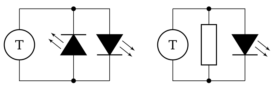
Depending on the circuit configuration (see Fig. 3), the brightness differs significantly. With two antiparallel LEDs, the light output is strongest because one LED conducts in each half-cycle of the signal. If only a single LED is used, the light output is weak because only one half of the signal contributes and the LED is mainly operated in reverse-bias. Interestingly, if both leads of the LED are touched with the hand, a reasonable brightness can be observed. The human body introduces finite resistance, which reduces the reverse-bias problem and yields better brightness than in the completely open case, but still not as good as in the antiparallel case.
Överkurs, technical excursion
To probe the acoustic field, a piezoelectric transducer is used as a receiver. The incident sound wave induces a periodic mechanical deformation of the piezoelectric crystal, which displaces charges in the lattice and generates an alternating voltage across the electrodes. Thus, electrically, the transducer behaves like a capacitive AC source with position-dependent amplitude. The circuit rapidly reaches a steady state in which the net transferred charge is zero, meaning that only alternating currents flow. Grounding one node does not change this behavior; it merely sets a DC reference potential without improving the signal or light output. Using antiparallel LEDs provides the most efficient use of the available current, as each half-cycle has a forward conduction path. Replacing a diode with a resistor introduces a bidirectional current path that diverts current away from the LED, reducing brightness. The resistance value is critical: a short circuit bypasses the LED completely, while an open circuit forces charge balance through the LED alone, where the very small reverse current severely limits the forward current and thus light output. Touching both terminals with the hand introduces moderate resistance for this scenario, allowing sufficient current for visible light, though still significantly less than in the antiparallel configuration.
b) Distance between antinodes
The transducer head is vertically moved and the approximate height change is recorded using the ruler. For a vertical distance of , the LEDs light up five times, starting and ending with lit up LEDs. Thus, five anti-nodes have been measured. This yields the estimate:
Grading scheme E1
| ID | Scoring Item | Points |
|---|---|---|
| E1-A1 | Correct circuit diagram (does mot require correct symbol for transducer or diode, but alternate polarity should be clearly indicated). | 0.5 pts |
| Second circuit diagram (with resistor/hands) | 0.3 pts | |
| Transducer and one diode only | 0.2 pts | |
| In case diode symbol without polarity is used, independent of remaining circuit | 0.1 pts | |
| Any circuit with a voltage source (power supply or levitator top rails): | 0.0 pts | |
| E1-B1 | Transducer head is moved along the z-axis and vertical distance between at least two anti-nodes is measured. | 0.2 pts |
| E1-B2 | Result for between adjacent antinodes is mm. | 0.3 pts |
| Total points | 1.0 pts |
Task E2: Acoustic levitator properties
a) Frequency of the transducers
The distance between two adjacent nodes is , where is the wavelength of the acoustic wave. Indeed, when one moves up, the phase of the sound wave from the transducers at the top part of the levitator decreases by , while the phase of the waves from the transducers at the bottom part increases by . This causes a total phase difference of .
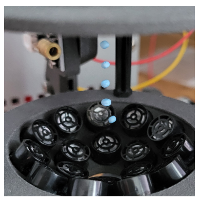
To determine the wavelength of the acoustic wave, one has to measure the location of the nodes. This can conveniently be achieved by levitating multiple beads of type (N) or (O). The advantage of the styrofoam beads (N) is that they are very light and hence deviate a little from the nodes (cf. task E3), while the advantage of the beads (O) is their regular shape. Levitating beads are shown in Fig. 4.
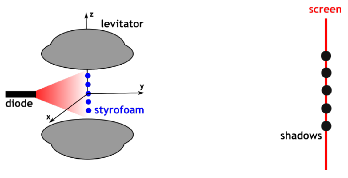
To magnify the image, illuminate the levitating beads with the red LED and project their shadows onto a screen, as shown in Figure 5. The magnification factor can, for example, be determined using a ruler in the following manner. One needs to place the ruler vertically in the center of the levitator, and determine the magnification factor from the distance between the projections of the vertical mm marks. Alternatively, the magnification factor can be deduced from the size of the shadow of beads (O) or (P), using that their real diameter is 2.0 mm. The described method for determining the magnification factor will be used in many of the subsequent tasks.
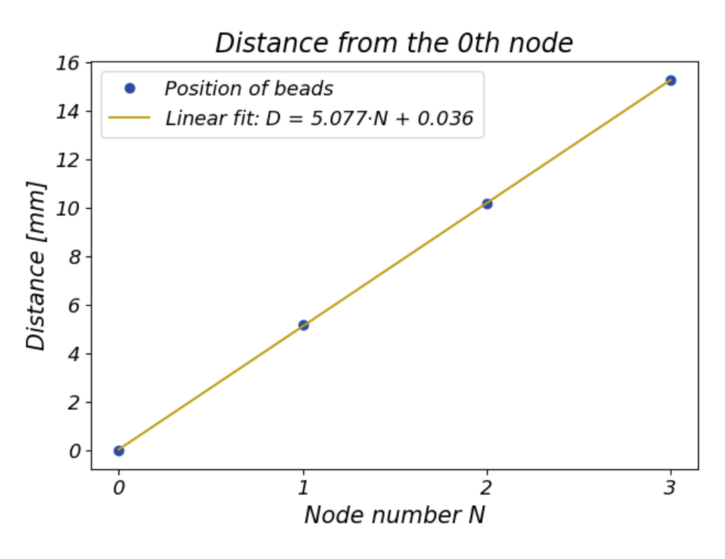
The obtained data are shown in Tab. 1, and Fig. 6 shows the distance from the 0:th bead as a function of the node number. The slope of the line is expected to be , and hence it is found that . Since , this gives:
| Node | Dist. on screen [cm] | Real dist. [mm] |
|---|---|---|
| 0 | 0.00 (reference) | 0.00 |
| 1 | 7.85 | 5.16 |
| 2 | 15.45 | 10.17 |
| 3 | 23.15 | 15.23 |
Table 1: Example data showing the distance of the nodes from the 0th node for magnification factor .
b) Mode X
When Mode X is turned on, a solid object placed in the acoustic field starts to move upward. This can be explained as follows. Let the wave produced by the lower half of the levitator, traveling along the positive axis, be given by . Similarly, let the wave produced by the upper half of the levitator, traveling along the negative axis, be given by , where is the slightly changed angular frequency. The resulting acoustic pressure is given by the sum of the two contributions:
where we used the relation . The sine term in this expression is a wave with the very long wavelength and the angular frequency , so it can be approximated as . The second term is almost a standing wave of wavelength , but with nodes moving with a small velocity , where . If , the nodes move in the direction of the negative axis, and if , they move along the positive axis. Using and we find that
Since levitating beads move along the positive axis when Mode X is on, it is deduced that . The value of can be found using Eq. 7, for example in the following way. First mark the position of the top part of a levitated bead’s shadow on the screen, as it levitates in two different nodes (as widely separated as possible, to increase accuracy). Place the bead slightly below the lowest of these nodes. Then turn on Mode X and measure the time it takes for the top part of the bead’s shadow to travel between the two marks on the screen. The frequency difference is found to be:
where was used. The results of a series of measurements for the travel time over a distance of four nodes are shown in Table 2. The average of 5.96 seconds on a distance of four nodes gives us .
Alternatively, one can describe the phenomenon by the Doppler effect in the system of reference moving with speed according to Eq. 9, where the nodes do not move relative to the ball. Therefore, the frequency from the upper and lower half would be measured to be the same in this reference frame.
Using that the ball is moving upward and the approximation one arrives at the relation in Eq. 10, where is the speed of the styrofoam bead and the speed of sound.
| Measurement | Time [s] |
|---|---|
| 1 | 5.84 |
| 2 | 6.00 |
| 3 | 5.94 |
| 4 | 5.96 |
| 5 | 6.06 |
| Average | 5.96 |
Table 2: One measurement series for the time it takes for a bead to travel a distance of four nodes.
Grading scheme E2
| ID | Scoring Item | Points |
|---|---|---|
| E2-A1 | Distance between nodes: | 0.2 pts |
| E2-A2 | Distance over three or four nodes measured OR PP/glass beads used in two nodes and argued for this choice using regular shape. | 0.3 pts |
| E2-A3 | GLOBAL: Magnification calibration method. Method statement, e.g., bead or ruler optically magnified, full points. Linearization and determining LED emission point ( 5 mm inside) awarded full points if done precisely. | 0.4 pts |
| E2-A4 | GLOBAL: Magnifying setup Sketch of an optical magnification setup. | 0.3 pts |
| E2-A5 | Measured raw vertical distance in magnified image (on ruler) 20 cm. For vertical distance 10 cm | 0.4 pts 0.2 pts |
| E2-A6 | Result for kHz (this interval should be rescaled accordingly if the answer in E2-A1 is wrong by a numerical factor). | 0.4 pts |
| E2-B1 | Correct theoretical derivation of formula (the derivation may assume that both plane waves have the same wavenumber ). If factor missing. | 0.5 pts 0.3 pts |
| E2-B2 | Phenomenon described, e.g., beads moving on the screen OR measuring the blinking frequency of a fixed LED with Mode X turned on. | 0.3 pts |
| E2-B3 | At least 5 time measurements with beads OR averaged over at least 10 blinkings of LED. for measurements, per measurement OR for each pair of blinkings, up to 10 blinkings | 0.5 pts 0.1 pts |
| E2-B4 | Using the formula | 0.1 pts |
| E2-B5 | Correct value Hz (should be rescaled accordingly if answer in E2-A1 is wrong by numerical factor) Hz | 0.4 pts 0.2 pts |
| E2-B6 | Correct sign of (negative) | 0.2 pts |
| Total points | 4.0 pts |
Överkurs
Task E3: Density of solid beads
The unknown material is polypropylene plastic (PP). Points can only be awarded for one of the methods A and B below. If both methods are attempted, the method yielding the highest total points is used.
Method A (deviation from node)
In this task, the same magnification approach as in Task E2 shall be used. However, the magnification should be made larger (since only one bead needs to be visible). A magnification of at least is obtained.
Start by finding the location of the node. A small piece of styrofoam is levitated approximately in the center of the node and marked on the screen.
According to the hint, the acoustic radiation force can be approximated by a spring force . The equation of force equilibrium for the levitated sphere is:
where is the mass of the bead, is the its density and is its volume. Using the assumption that the acoustic pressure is proportional to the voltage it is clear that .
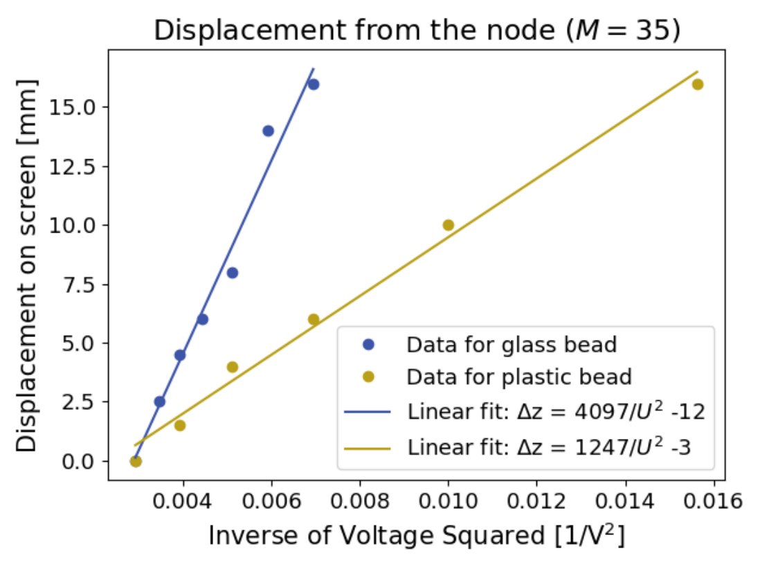
Since the glass and plastic beads have the same shape and size, the slope of the obtained line for vs. is proportional to the density of the levitated object. Thus, it follows that
The glass is levitated at the maximum voltage and the offset from the node is measured (on the screen, the image is magnified) for different voltages. At least five measurement points are required to get accurate results. The measurements are repeated for the plastic bead. From the slope of the vs. -graphs in Fig. 8 the densities are calculated according to Eq. 13.
Grading scheme E3: method A (deviation from node)
| ID | Scoring Item | Points |
|---|---|---|
| E3-A1 | Correct force balance (one version enough, not grading sign). | 0.3 pts |
| E3-A2 | gives the density of PP (or if pairwise measurements for constant voltage, ratio of displacements). | 0.5 pts |
| E3-A3 | Magnification factor 30 or if diode the closest possible to levitator distance from node to screen 66 cm. Magnification factor 20 or if diode the closest possible to levitator distance from node to screen 43 cm | 0.4 pts 0.2 pts |
| E3-A4 | At least 4 voltage and displacement measurements for glass bead (the voltage may be the same for all measurements). For 3 measurements. For 2 measurements. For 1 measurements | 0.5 pts 0.3 pts 0.2 pts 0.1 pts |
| E3-A5 | At least 4 voltage for plastic bead (the voltage may be the same for all measurements). For 3 measurements. For 2 measurements. For 1 measurements | 0.5 pts 0.3 pts 0.2 pts 0.1 pts |
| E3-A6 | Graphical evaluation (slope) for both materials OR linear regression on calculator. Point-wise average yields no points, unless clearly stated that the exact location of the node is determined (e.g. by levitating a styrofoam bead at a high voltage in the same node, marking the position on the screen). | 0.4 pts |
| E3-A7 | Density within the interval | 0.4 pts |
| Total points | 3.0 pts |
Method B (drop voltage)
An alternative method to compare the densities of the beads of type (O) and (P) is to analyze the drop voltage, i.e. the smallest voltage at which the beads can be levitated. Indeed, by levitating at different voltages, one notices that denser objects require a higher voltage to be levitated.
The approach is based on the observation that a levitating spherical bead of a fixed size will fall precisely when its deviation from the node, , reaches a certain value , independent of the bead's density. At this point, the acoustic force reaches a maximum, so a further increase of only results in a lower restoring force. If one considers the restoring acoustic force as a spring this corresponds, in some sense, to the spring breaking.
According to the theory presented in the task, the acoustic force on a bead of a fixed shape at the deviation is given by , where is a constant. Hence, the drop voltage satisfies
where is the volume of the bead. Thus, we conclude that
The plastic and glass bead are levitated in the central node. The voltage is slowly decreased and the drop voltage is recorded. At least three measurements should be done for the drop voltage of each bead type. The average drop voltage is used to calculate the density of the plastic bead according to Eq. 15. Alternatively, it could be argued that the minimum of the recorded drop voltage values should be used. Indeed, due to the shaking of the bead, it may fall at a voltage higher than , and therefore should be best approximated by the minimum voltage of the recorded values.
Some example data is shown in Tab. 3 and the density result based on the example data is:
| [V] | [V] | |
|---|---|---|
| 11.1 | 7.1 | |
| 11.1 | 7.1 | |
| 11.1 | 7.0 | |
| 11.0 | 7.1 | |
| 11.1 | 7.0 | |
| Average: | 11.08 | 7.04 |
Table 3: Example data showing drop voltage for glass and plastic bead.
Grading scheme E3: method B (drop voltage)
| ID | Scoring Item | Points |
|---|---|---|
| E3-B1 | Idea that the drop voltage is influenced by the density of the beads. | 0.5 pts |
| E3-B2 | Idea that there is a maximum displacement for which the beads fall. | 0.5 pts |
| E3-B3 | Correct force balance or | 0.3 pts |
| E3-B4 | Idea that gives the density | 0.3 pts |
| E3-B5 | At least 3 voltage measurements for glass bead. For 2 voltage measurements. For 1 voltage measurements | 0.5 pts 0.3 pts 0.1 pts |
| E3-B6 | At least 3 voltage measurements for plastic bead. For 2 voltage measurements. For 1 voltage measurements | 0.5 pts 0.3 pts 0.1 pts |
| E3-B7 | Correct density within range | 0.4 pts |
| Total points | 3.0 pts |
Överkurs
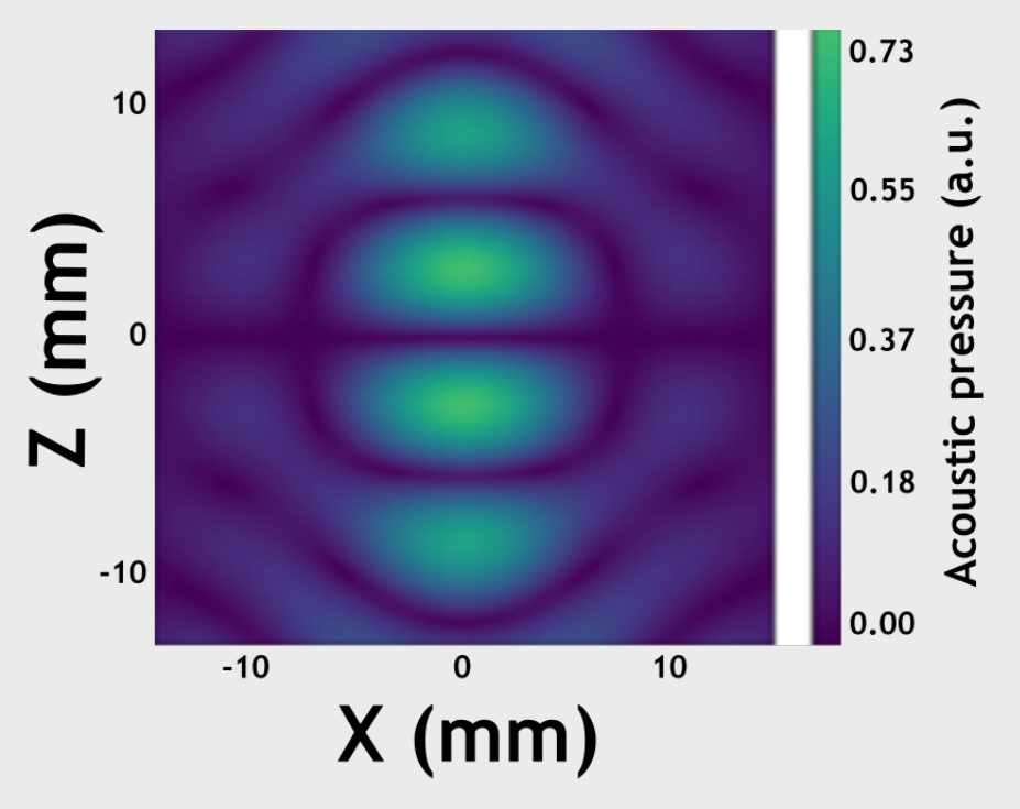
- The distance between two adjacent nodes is (NB! this is not the wavelength of the acoustic force in blue, which is ). See Fig. 9 for a sketch of acoustic pressure force. As in described in method B, there is a point where an increase in the displacement does not give an increase in the acoustic force. This corresponds to a spring becoming permanently deformed. This happens at .
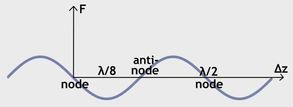
- There is a comparatively simple formula describing the acoustic force on a spherical bead whose radius is much smaller than the wavelength of the ultrasound:
Here is a dimensionless contrast factor depending on the compressibilities and densities of the bead and the ambient air, is the wavenumber, and is the acoustic energy density. In this task, however, it is not accurate to assume that the droplets are much smaller than the wavelength, and the dependence is more complicated.
Task E4: Evaporation
The liquid I in question is isopropanol (IPA).
a) Evaporation constant
The given evaporation model states that the squared diameter of the droplet decreases linearly with time. To measure evaporation, one has to calibrate the setup in a similar manner as in E2. Since the given equation holds for spherical droplets, one has to convert the ellipsoidal shape to a sphere, according to , i.e. , where we used (by symmetry). This can be written in terms of the diameter as where is the semi-major axis and is the semi-minor axis of the ellipsoidal droplet. To estimate , measure the major and minor axes and wait in between measurements. The task asks to determine when () so data are collected when the droplet is both larger and slightly smaller than this size (for task E4b). One has to convert the results first to the observed diameter with and then to the real diameter with , where is the magnification factor. An example dataset is shown in Tab. 4 and visualized in Fig. 10.
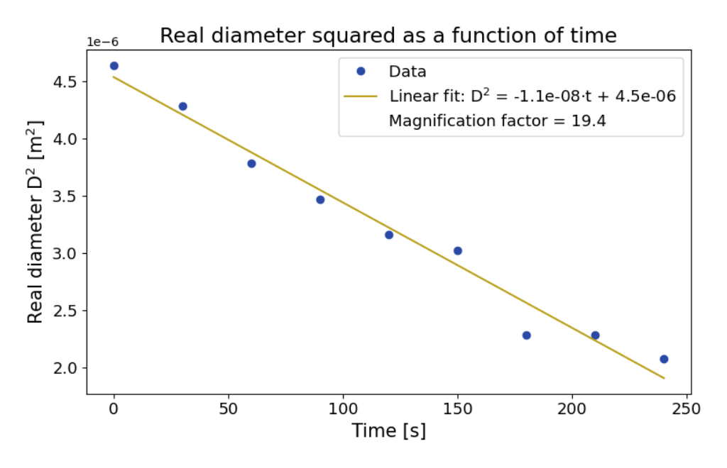
The value of is then read as the slope of the curve which gives us the result:
b) Evaporation time
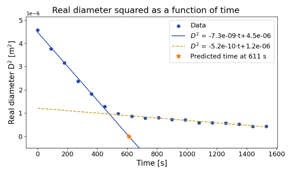
When one waits long enough one can observe that the evaporation rate slows down considerably when a certain size is reached. In Figure 11 one sees that this happens after 600 seconds at about . We see that a prediction based on the first slope would have led to a drastic underestimation of the evaporation time.
| Time [s] | Major [mm] | Minor [mm] | Diameter [mm] | Real [m²] |
|---|---|---|---|---|
| 0 | 47 | 33 | 4.2e+01 | 4.6e-06 |
| 30 | 45 | 32 | 4.0e+01 | 4.3e-06 |
| 60 | 41 | 32 | 3.8e+01 | 3.8e-06 |
| 90 | 39 | 31 | 3.6e+01 | 3.5e-06 |
| 120 | 37 | 30 | 3.5e+01 | 3.2e-06 |
| 150 | 37 | 28 | 3.4e+01 | 3.0e-06 |
| 180 | 30 | 28 | 2.9e+01 | 2.3e-06 |
| 210 | 30 | 28 | 2.9e+01 | 2.3e-06 |
| 240 | 29 | 26 | 2.8e+01 | 2.1e-06 |
Table 4: Example data showing time for the measurement, on screen major axis, on screen minor axis, diameter of the corresponding sphere on the screen and the real, actual diameter of the droplet squared. The scale factor for this measurement was 20.
Grading scheme E4
| ID | Scoring Item | Points |
|---|---|---|
| E4-A1 | Both major axis and minor axis measured. | 0.3 pts |
| E4-A2 | At least 9 data points for , with at least 20 s between the measurements (if initial determined from volume measured using the inaccurate scale of the syringe, no points). — at least 7 data points 0.5 pts — at least 5 data points 0.3 pts — at least 3 data points 0.1 pts | 0.7 pts |
| E4-A3 | Measuring the droplet for a total time of at least 4 min = 240 s above . | 0.2 pts |
| E4-A4 | Diameter of corresponding sphere calculated correctly . | 0.2 pts |
| E4-A5 | Magnification — Magnification 0.1 pts | 0.2 pts |
| E4-A6 | Correct linearization (integrated version of Eq. 3 against or idea to plot against ). | 0.2 pts |
| E4-A7 | Determining as the slope, graphically or by using a linear regression on calculator, of recorded data vs. . | 0.2 pts |
| E4-A8 | Value of . | 0.5 pts |
| E4-B1 | Observation that the droplet's evaporation slows down when a certain size is reached. | 0.3 pts |
| E4-B2 | Statement that the result in part a) would have led to an underestimation of the evaporation time. | 0.2 pts |
| Total points | 3.0 pts |
Överkurs
- The relation is known as the D-squared law, and it is typically assumed to hold for small spherical droplets. In this problem we have applied it explicitly to non-spherical droplets by converting the axes to an equivalent diameter and found out that it still holds.
- Evaporation is a phenomenon that is affected by a lot of variables. The D-square law is a simple but a useful tool to describe the phenomenon. Its downside is that it does not take into account differences caused by temperature, humidity, air pressure, shape of the droplet, draft or turbulence by the acoustic field. We have tried to take into account these effects by measuring in different conditions which has lead to a large interval of accepted solutions.
- Observe the strong change in the value of when we finally get to aspect ratio 1, i.e., the ratio between the major axis and the minor axis, equaling to 1. This shows that the used model is too simple to explain the full range of the phenomena. The moral of the problem can be summarized by the words of George Box: "All models are wrong, but some are useful."
Task E5: Surface tension
a) Surface tension ranking
One can quickly determine which of the liquids has a lower surface tension in a number of ways. One idea is to just place two similarly big droplets of the liquids on the table surface and visually notice that the contact angle for liquid I is much lower. Another approach is to levitate similarly big droplets in the levitator and deform them or make them explode and note that this happens at significantly lower voltages for liquid I. Alternatively, just solving Task b) quantitatively also gives the right qualitative answer.
b) Unknown surface tension
The shape of a droplet only depends on its volume and the ratio but in an unknown manner. To solve the task, we can measure pairs of droplets (one of each liquid) with equal volume and apply a voltage such that their shape matches. This implies
Experimentally, the already established magnification setup is used and we start levitating a droplet of liquid II and deform it at voltage such that it is clearly non-spherical. For a precise measurement of , it is necessary to significantly deform the droplet because otherwise the contribution of to the overall shape becomes too small. We mark the shape of the droplet on the screen. Next, we remove the droplet from the levitator and now levitate a droplet of liquid I with the same volume. We tune the voltage of the levitator such that the shape matches our markings made before and write down this voltage as well. To get a droplet of the same volume, it is a good strategy to levitate a slightly larger droplet at first and then wait a bit and use the (previously explored) evaporation to fine-tune the volume to match the shape exactly.
Finally, the surface tension can be determined via the known surface tension as:
and we repeat the measurement 5 times to increase our accuracy.
| [V] | [V] | [mN/m] |
|---|---|---|
| 16.3 | 9.6 | 25.3 |
| 17.8 | 10.3 | 24.4 |
| 14.3 | 8.5 | 25.8 |
| 16.4 | 9.7 | 25.5 |
| 15.6 | 9.0 | 24.3 |
Grading scheme E5
| ID | Scoring Item | Points |
|---|---|---|
| E5-A1 | Effective idea to compare the surface tension. | 0.2 pts |
| E5-A2 | Correct conclusion . | 0.3 pts |
| E5-B1 | Idea to use symmetry i.e., and same droplet shapes (pairwise at least). If contact angle approach used without magnification , no poits are awarded for the entire task E5b | 0.5 pts |
| E5-B2 | Obtaining or using | 0.2 pts |
| E5-B3 | Repeating the correct measurement procedure (evidenced by pairs of voltages) for 5 repetitions. — For at least 3 repetitions 0.2 pts — For at least 1 repetitions 0.1 pts | 0.3 pts |
| E5-B4 | Result for within — 0.5 pts — 0.2 pts | 1.0 pts |
| Total points | 2.5 pts |
Överkurs
- Liquid I is IPA (isopropanol), which has a surface tension of 21.8 mN/m according to the literature. The method overestimates the surface tension slightly but is reasonably accurate considering the measurement technique.
Task E6: Explosion
a) Fitting parameters
Measure the explosion voltage for droplets of different equivalent diameters . By Equation (4), a plot of against is expected to yield a straight line, and the constants and are determined as the slope and -intercept of this line, respectively. The obtained data is presented in Table 5, and the corresponding plot is shown in Figure 12. The obtained values for and are:
To determine the equivalent diameter of a levitated droplet, use the technique described in Task E4. Note that the approximation of a droplet as an ellipsoid is most accurate when the droplet is round, so the diameter of the droplet should be measured at a comparatively low voltage. To reduce the evaporation of the droplet between its explosion and the diameter measurement, one needs to quickly increase the voltage to a moderately high value, guided by the shape of the droplet. Then change the voltage by 0.1 V at a time until the droplet explodes. Often, when a large droplet explodes, the remains form a smaller droplet, which can be used for the next measurement, to conveniently obtain a large variation of values.
| [mm] | [mm] | [mm] | [mm] | [V] | [V] |
|---|---|---|---|---|---|
| 73 | 63 | 1.70 | 0.590 | 17.7 | 313.3 |
| 87 | 65 | 1.93 | 0.519 | 15.9 | 252.8 |
| 78 | 68 | 1.82 | 0.550 | 16.7 | 278.9 |
| 140 | 71 | 2.72 | 0.367 | 13.2 | 174.2 |
| 122 | 62 | 2.38 | 0.421 | 14.1 | 198.8 |
| 99 | 59 | 2.03 | 0.492 | 15.6 | 243.4 |
| 102 | 70 | 2.19 | 0.456 | 14.6 | 213.2 |
| 80 | 52 | 1.69 | 0.592 | 17.5 | 306.3 |
| 142 | 66 | 2.68 | 0.373 | 13.1 | 171.6 |
| 117 | 72 | 2.43 | 0.412 | 13.8 | 190.4 |
| 113 | 67 | 2.32 | 0.432 | 14.6 | 213.2 |
| 87 | 52 | 1.79 | 0.559 | 16.7 | 278.9 |
| 165 | 87 | 3.25 | 0.308 | 12.5 | 156.3 |
Table 5: Data corresponding to the measurements of exploding droplets. The axes of the droplet are measured in mm on the screen. The magnification is 41.
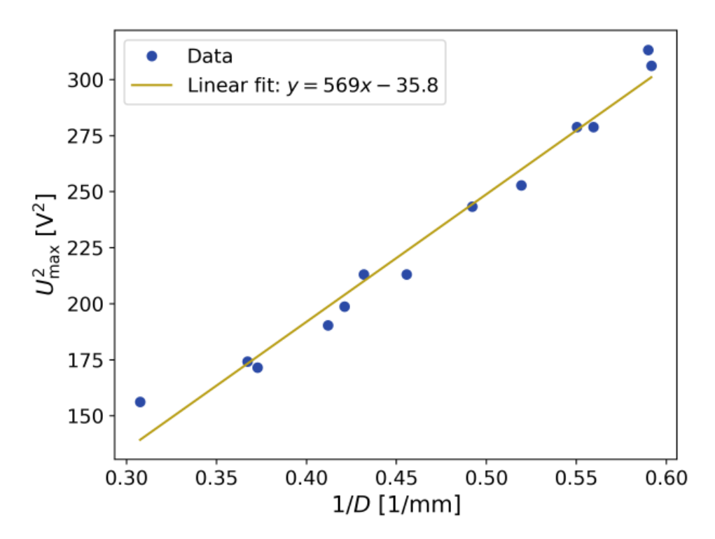
b) Maximum diameter to levitate
In this task, two effects preventing the droplet from levitating are considered:
- If the applied voltage is too high, the droplet explodes, as analysed in the previous subtask. This yields an upper bound for the voltage, decreasing with .
- If the applied voltage is too low, the droplet falls. This yields a lower bound , increasing with .
An estimate of the equivalent diameter of the largest droplet that can be levitated is obtained as the intersection of the two curves corresponding to the above restrictions. The explosion voltage was analyzed in the previous subtask, so what remains to understand is the dependence between and . Note that small droplets can be created by exploding larger droplets, as in the previous subtask. The recorded measurement values are presented in Table 6, and and are plotted against in Figure 13.
| [mm] | [mm] | [mm] | [V] |
|---|---|---|---|
| 99 | 76 | 2.61 | 8.7 |
| 87 | 69 | 2.32 | 8.4 |
| 124 | 80 | 3.08 | 10.0 |
| 121 | 82 | 3.07 | 9.9 |
| 63 | 58 | 1.77 | 7.7 |
| 74 | 61 | 1.99 | 8.0 |
| 54 | 45 | 1.47 | 7.7 |
| 86 | 65 | 2.26 | 8.9 |
| 125 | 83 | 3.14 | 10.1 |
| 124 | 84 | 3.14 | 10.0 |
| 114 | 85 | 2.97 | 9.6 |
| 80 | 60 | 2.09 | 8.0 |
| 111 | 77 | 2.82 | 9.3 |
| 83 | 62 | 2.17 | 8.1 |
| 148 | 81 | 3.48 | 11.0 |
| 134 | 76 | 3.19 | 10.1 |
| 69 | 54 | 1.83 | 7.7 |
| 58 | 49 | 1.58 | 7.2 |
| 105 | 69 | 2.63 | 8.9 |
| 89 | 62 | 2.27 | 8.2 |
Table 6: Data corresponding to the measurements of drop voltages. The axes of the droplet are measured in mm on the screen. The magnification is 35.
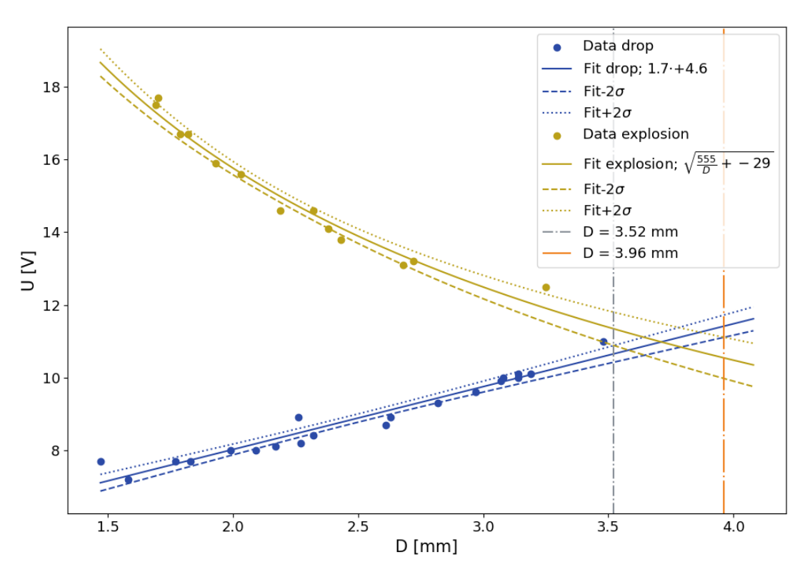
As seen in the figure, the fall voltage is described fairly well by an affine linear function, i.e., . Hence, by Equation (4), is obtained by solving
This equation can, for example, be solved graphically or by using the bisection method. It is found that
which is the desired result.
Grading scheme E6
| ID | Scoring Item | Points |
|---|---|---|
| E6-A1 | Correct linearization (, the idea that a plot of against has slope and -intercept ). A table with and data suffices as evidence to get these points. | 0.4 pts |
| E6-A2 | At least 10 data points measured for the explosion curve (if volume measured using the inaccurate scale of the syringe, no points shall be awarded here). | 0.5 pts |
| At least 8 data points | 0.4 pts | |
| At least 6 data points | 0.3 pts | |
| At least 4 data points | 0.2 pts | |
| At least 2 data points | 0.1 pts | |
| E6-A3 | Values of span at least 1 mm. | 0.3 pts |
| E6-A4 | Correct value: .; | 0.4 pts; 0.2 pts |
| E6-A5 | Correct value: .; | 0.4 pts; 0.2 pts |
| E6-B1 | Idea that the maximum droplet size is found at the intersection of the fall curve and the explosion curve. | 0.5 pts |
| E6-B2 | At least 10 data points measured for the drop voltage (if volume measured using the inaccurate scale of the syringe, no points shall be awarded here). | 0.5 pts |
| At least 8 data points | 0.4 pts | |
| At least 6 data points | 0.3 pts | |
| At least 4 data points | 0.2 pts | |
| At least 2 data points | 0.1 pts | |
| E6-B3 | Values of span at least 1 mm. | 0.2 pts |
| E6-B4 | At least one point with measured. | 0.1 pts |
| E6-B5 | Reasonable method for determining intersection of and (for example a graphical solution or the bisection method). | 0.3 pts |
| E6-B6 | Maximum diameter | 0.4 pts |
| Total points | 4.0 pts |
Task E7: Mysterious line
The horizontal line is formed when the droplet is quite flat, typically around before reaching the explosion voltage. For imperfect alignment (adjustable via the hex-screws) the line might also appear below or above the droplet. In Fig. 14, you can see an image of the phenomenon.
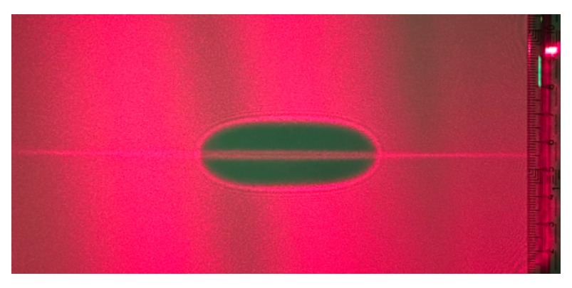
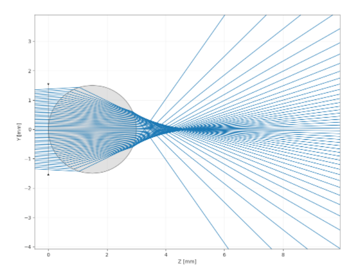
To break the optical effect of the droplet down, it can be modeled as the superposition of two plano-convex lenses with liquid in between them in the vertical cross-section and a round (cylindrical) lens in the horizontal cross section.
The line emerges when incident rays from the diode propagating in the vertical plane are focused to a point on the screen, as shown in the simulation in Fig. 17. Since the dimensions of the droplet are much smaller than all other relevant distances, both the incident and emergent rays are approximately parallel to the optic axis. Hence, the situation in Figure 17 is obtained when the length of the droplet is
where is the focal length of the lenses in the vertical direction. The ray propagation inside the droplet can be seen in Figure 15.
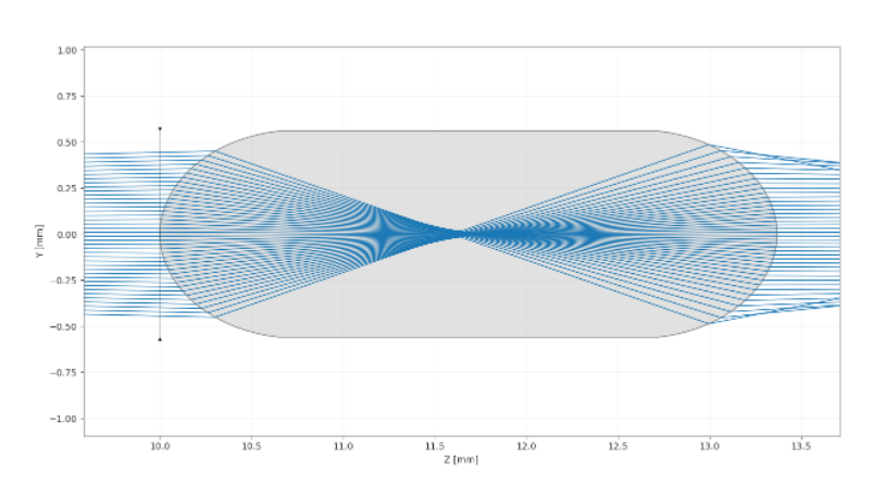
This observation is used to determine the index of refraction of the analyzed liquid. Note that the focal length is given by , where is the radius of curvature of the two lenses in the vertical plane (near the tip of the droplet). Hence, by Eq. (20), the index of refraction of the liquid can be determined as
One way of determining the radius of curvature of one of the lenses is the following. First sketch the contour of the levitating droplet when the line is visible. Then draw two lines perpendicular to the contour near the vertical center of the droplet. The distance from the outermost point of the droplet to the point of intersection of these two lines is . This is shown in Fig. 16. This measurement is repeated a number of times to increase the precision of the result. The final result is then the average of the single measurements.
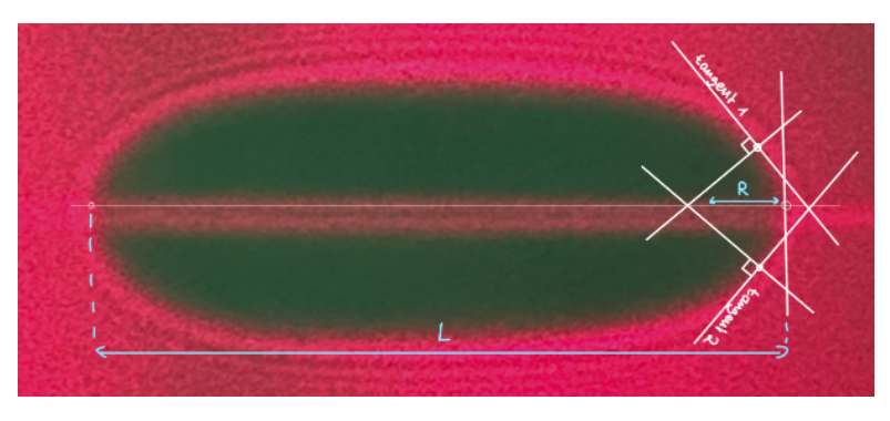
| L [cm] | R [cm] | n |
|---|---|---|
| 15.2 | 2.2 | 1.41 |
| 21.2 | 2.45 | 1.30 |
| 17.5 | 2.2 | 1.34 |
| 17.5 | 2.0 | 1.30 |
| 19.7 | 2.7 | 1.38 |
Table 7: Experimental data for E7
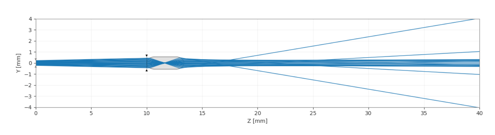
Due to the refraction in the horizontal direction, a line is formed instead of a point, as shown in the simulation in Fig. 18.
Överkurs
- The unknown red liquid is water with some red food dye.
- The explanation given above suggests that the line should be visible only when the length of the droplet and the radius of curvature match perfectly. Hence, one could expect it to be very hard to observe the line phenomenon in practice. However, the conditions are somewhat relaxed due to aberrations of the two lenses. The incident rays are not focused into a single point, but rather into a short interval, and this allows for some flexibility in the constraints. The phenomenon is similar to an astigmatic lens.
- When light passes through the droplet and forms a shadow, Fraunhofer diffraction causes the light to spread and interfere, producing bright and dark fringes around the shadow rather than a perfectly sharp edge. The effect becomes more noticeable when the droplet size is small or when the observation screen is far from the droplet. This makes the apparent edge position depend on the measurement setup and potentially introduces systematic errors in the estimated droplet size.
Grading scheme E7
| ID | Scoring Item | Points |
|---|---|---|
| E7-1 | Vertical contribution: Idea that line is formed when , together with sketch as in Fig. 15. Ray propagation physically correct. Symmetry stated by text or labeling similar angles. | 0.8 pts |
| E7-2 | Horizontal contribution: Explain why line is formed instead of point, Fig. 18. Labeled. Idea to split into vertical and horizontal contribution | 0.4 pts / 0.2 pts |
| E7-3 | Correct relation OR using Snell's law and clearly indicating relevant angles (both only if E7-1 was awarded). Incorrect relation - using the lensmaker's formula, forgetting second half of lens is liquid (if E7-1 awarded) | 0.4 pts / 0.1 pts |
| E7-4 | Physically possible method for estimating , reasonable value of obtained (). | 0.4 pts |
| E7-5 | At least 3 measurements (measurements consist of pairs OR angles for Snell's law). At least 2 measurements. At least 1 measurement. | 0.3 pts / 0.2 pts / 0.1 pts |
| E7-6 | Refractive index . | 0.2 pts |
| Total points | 2.5 pts |
E8 Experimental Techniques
Grading scheme E8
| ID | Scoring Item | Points |
|---|---|---|
| E8-1 | The box of the experimental setup is torn into pieces | -0.2 pts |
| E8-2 | A LED is broken/blown up. Per LED broken. | -0.1 pts |
| E8-3 | Some equipment is missing. | -0.1 pts |
| E8-4 | The electrical control box is broken | -0.1 pts |
| Total points | -0.5 pts |
Оригинал в Архива: eupho2026_experiment_problems.pdf · официални решения: eupho2026_experiment_solutions.pdf